Construction of Quantile-Quantile and Probability Plots

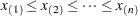
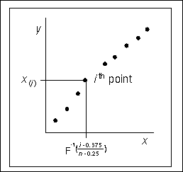
Figure 5.20.6 illustrates how a Q-Q plot is constructed. First, the nonmissing values of the variable are ordered from smallest to largest:

Then the th ordered value is represented on the plot by a point whose -coordinate is and whose -coordinate is , where is the theoretical distribution with zero location parameter and unit scale parameter.

Output 5.20.6 Construction of a Q-Q Plot

You can modify the adjustment constants and with the RANKADJ= and NADJ= options. This default combination is recommended by Blom (1958). For additional information, refer to Chambers et al. (1983). Since is a quantile of the empirical cumulative distribution function (ecdf), a Q-Q plot compares quantiles of the ecdf with quantiles of a theoretical distribution. Probability plots (see PROBPLOT Statement) are constructed the same way, except that the -axis is scaled nonlinearly in percentiles.