Creating a Normal Quantile-Quantile Plot

[See CAPQQ1 in the SAS/QC Sample Library]Measurements of the distance between two holes cut into 50 steel sheets are saved as values of the variable Distance in the following data set:

data Sheets;
   input Distance @@;
   label Distance='Hole Distance in cm';
   datalines;
 9.80 10.20 10.27  9.70  9.76
10.11 10.24 10.20 10.24  9.63
 9.99  9.78 10.10 10.21 10.00
 9.96  9.79 10.08  9.79 10.06
10.10  9.95  9.84 10.11  9.93
10.56 10.47  9.42 10.44 10.16
10.11 10.36  9.94  9.77  9.36
 9.89  9.62 10.05  9.72  9.82
 9.99 10.16 10.58 10.70  9.54
10.31 10.07 10.33  9.98 10.15
;
run;

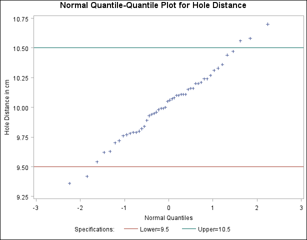
The cutting process is in control, and you decide to check whether the process distribution is normal. The following statements create a Q-Q plot for Distance, shown in Figure 5.20.2, with lower and upper specification lines at 9.5 cm and 10.5 cm:¹

symbol v=plus;
title 'Normal Quantile-Quantile Plot for Hole Distance';
proc capability data=Sheets noprint;
   spec lsl=9.5 usl=10.5;
   qqplot Distance;
run;

The plot compares the ordered values of Distance with quantiles of the normal distribution. The linearity of the point pattern indicates that the measurements are normally distributed. Note that a normal Q-Q plot is created by default. The specification lines are requested with the LSL= and USL= options in the SPEC statement.

Output 5.20.2 Normal Quantile-Quantile Plot Created with Traditional Graphics