Example 5.12 Computing Kernel Density Estimates

[See CAPKERN1 in the SAS/QC Sample Library]This example illustrates the use of kernel density estimates to visualize a nonnormal data distribution.

The effective channel length (in microns) is measured for 1225 field effect transistors. The channel lengths are saved as values of the variable Length in a SAS data set named Channel:

data Channel;
   length Lot $ 16;
   input Length @@;
   select;
        when (_n_ <= 425) Lot='Lot 1';
        when (_n_ >= 926) Lot='Lot 3';
        otherwise Lot='Lot 2';
     end;
   datalines;
0.91 1.01 0.95 1.13 1.12 0.86 0.96 1.17 1.36 1.10
0.98 1.27 1.13 0.92 1.15 1.26 1.14 0.88 1.03 1.00
0.98 0.94 1.09 0.92 1.10 0.95 1.05 1.05 1.11 1.15
1.11 0.98 0.78 1.09 0.94 1.05 0.89 1.16 0.88 1.19

   ... more lines ...   

1.80 2.35 2.23 1.96 2.16 2.08 2.06 2.03 2.18 1.83
2.13 2.05 1.90 2.07 2.15 1.96 2.15 1.89 2.15 2.04
1.95 1.93 2.22 1.74 1.91
;

When you use kernel density estimates to explore a data distribution, you should try several choices for the bandwidth parameter since this determines the smoothness and closeness of the fit. You can specify a list of C= values with the KERNEL option to request multiple density estimates, as shown in the following statements:

title "FET Channel Length Analysis";
proc capability data=Channel noprint;
   histogram Length / kernel(c = 0.25 0.50 0.75 1.00);
run;

The L= option specifies distinct line types for the curves (the L= values are paired with the C= values in the order listed). The display, shown in Output 5.12.1, demonstrates the effect of . In general, larger values of yield smoother density estimates, and smaller values yield estimates that more closely fit the data distribution.

Output 5.12.1 Multiple Kernel Density Estimates

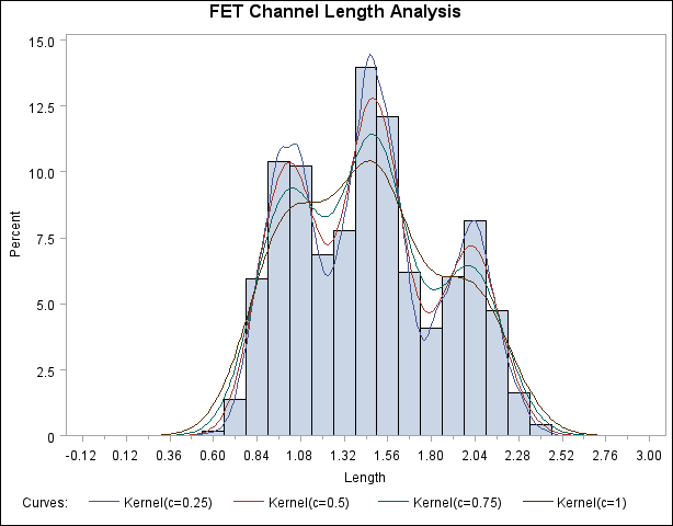
Output 5.12.1 reveals strong trimodality in the data, which are explored further in Creating a One-Way Comparative Histogram.