specifies the shape parameter for fitted curves requested with the BETA and GAMMA options. Enclose the ALPHA= option in parentheses after the BETA or GAMMA options. If you do not specify a value for , the procedure calculates a maximum likelihood estimate. See Example 5.8. You can specify A= as an alias for ALPHA= if you use it as a beta-option. You can specify SHAPE= as an alias for ALPHA= if you use it as a gamma-option.

[Traditional Graphics] displays labels above the histogram bars. If you specify BARLABEL=COUNT, the label shows the number of observations associated with a given bar. BARLABEL=PERCENT shows the percent of observations represented by that bar. If you specify BARLABEL=PROPORTION, the label displays the proportion of observations associated with the bar.

[Traditional Graphics] specifies the width of the histogram bars in screen percent units.

displays a fitted beta density curve on the histogram. The curve equation is

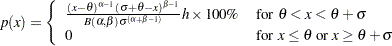
where and

lower threshold parameter (lower endpoint parameter)
scale parameter
shape parameter
shape parameter
width of histogram interval

The beta distribution is bounded below by the parameter and above by the value . You can specify and by using the THETA= and SIGMA= beta-options. The following statements fit a beta distribution bounded between 50 and 75 by using maximum likelihood estimates for and :

proc capability;
   histogram length / beta(theta=50 sigma=25);
run;

In general, the default values for THETA= and SIGMA= are 0 and 1, respectively. You can specify THETA=EST and SIGMA=EST to request maximum likelihood estimates for and .

The beta distribution has two shape parameters, and . If these parameters are known, you can specify their values with the ALPHA= and BETA= beta-options. If you do not specify values, the procedure calculates maximum likelihood estimates for and .

The BETA option can appear only once in a HISTOGRAM statement. Table 5.18 lists secondary options you can specify with the BETA option. See Example 5.8. Also see Formulas for Fitted Curves.

specifies the second shape parameter for beta density curves requested with the BETA option. Enclose the BETA= option in parentheses after the BETA option. If you do not specify a value for , the procedure calculates a maximum likelihood estimate. See Example 5.8.

[Traditional Graphics] specifies the fill color for a box-and-whisker plot in a bottom margin requested with the BMPLOT= option. By default, the box-and-whisker plot is not filled.

[Traditional Graphics] specifies the color for filling the frame of a bottom margin plot requested with the BMPLOT= option. By default, this area is not filled.

[Traditional Graphics] specifies the color of a carpet plot or dot plot, or the outline color of a box-and-whisker plot, in a bottom margin plot requested with the BMPLOT= option.

[Traditional Graphics] specifies the height in screen percentage units of a bottom margin plot requested with the BMPLOT= option. By default, a bottom margin plot occupies 15 percent of the vertical display space.

[Traditional Graphics] produces a carpet plot, dot plot, or box-and-whisker plot along the bottom margin of a histogram. A carpet plot or dot plot shows the distribution of individual observations along the histogram’s horizontal axis. A carpet plot represents each observation with a vertical line. A dot plot marks each observation with a symbol. A box-and-whisker plot gives a summary of the data distribution that a histogram alone does not provide. The left and right edges of the box are located at the first and third quartiles. A central vertical line is drawn at the median and a symbol is plotted inside the box at the mean. If you specify the SKELETAL keyword, a box-and-whisker plot is produced with whiskers extending to the minimum and maximum values. If you specify SCHEMATIC, a schematic box-and-whisker plot is produced. In a schematic box-and-whisker plot, the whiskers extend to the smallest value within the lower fence and the largest value within the upper fence. Fences are defined in terms of the interquartile range (IQR). The lower fence is 1.5 IQR below the first quartile and the upper fence is 1.5 IQR above the third quartile. Each observation outside the fences is plotted with a symbol.

specifies the shape parameter for Weibull density curves requested with the WEIBULL option. Enclose the C= option in parentheses after the WEIBULL option. If you do not specify a value for , the procedure calculates a maximum likelihood estimate. See Example 5.9. You can specify the SHAPE= option as an alias for the C= option.

specifies the standardized bandwidth parameter for kernel density estimates requested with the KERNEL option. Enclose the C= option in parentheses after the KERNEL option. You can specify up to five values to request multiple estimates. You can also specify the C=MISE option, which produces the estimate with a bandwidth that minimizes the approximate mean integrated square error (MISE). For example, the following statements compute three density estimates:

proc capability;
   histogram length / kernel(c=0.5 1.0 mise);
run;

The first two estimates have standardized bandwidths of 0.5 and 1.0, respectively, and the third has a bandwidth that minimizes the approximate MISE.

You can also use the C= option with the K= option, which specifies the kernel function, to compute multiple estimates. If you specify more kernel functions than bandwidths, the last bandwidth in the list is repeated for the remaining estimates. Likewise, if you specify more bandwidths than kernel functions, the last kernel function is repeated for the remaining estimates. For example, the following statements compute three density estimates:

proc capability;
   histogram length / kernel(c=1 2 3 k=normal quadratic);
run;

The first uses a normal kernel and a bandwidth of 1, the second uses a quadratic kernel and a bandwidth of 2, and the third uses a quadratic kernel and a bandwidth of 3. See Example 5.12.

If you do not specify a value for , the bandwidth that minimizes the approximate MISE is used for all the estimates.

[Traditional Graphics] specifies the color of the outline of histogram bars. This option overrides the C= option in the SYMBOL1 statement.

[Traditional Graphics] specifies a color used to fill the bars of the histogram (or the area under a fitted curve if you also specify the FILL option). See the entries for the FILL and PFILL= options for additional details. See Figure 5.7.5 and Output 5.8.1. Refer to SAS/GRAPH: Reference for a list of colors. By default, bars are filled with an appropriate color from the ODS style.

[Traditional Graphics] specifies the color for grid lines requested with the GRID option. By default, grid lines are the same color as the axes. If you use CGRID=, you do not need to specify the GRID option.

[Traditional Graphics] draws reference lines requested with the HREF= and VREF= options behind the histogram bars. By default, reference lines are drawn in front of the histogram bars.

[Traditional Graphics] specifies that histogram bars are clipped at the upper and lower specification limit lines when there are no observations outside the specification limits. The bar intersecting the lower specification limit is clipped if there are no observations less than the lower limit; the bar intersecting the upper specification limit is clipped if there are no observations greater than the upper limit. If you specify CLIPSPEC=CLIP, the histogram bar is truncated at the specification limit. If you specify CLIPSPEC=NOFILL, the portion of a filled histogram bar outside the specification limit is left unfilled. Specifying CLIPSPEC=NOFILL when histogram bars are not filled has no effect.

specifies the name of a LEGEND statement describing the legend for specification limits and fitted curves. Specifying CURVELEGEND=NONE suppresses the legend for fitted curves; this is equivalent to specifying the NOCURVELEGEND option.

specifies the first shape parameter for Johnson and Johnson density curves requested with the SB and SU options. Enclose the DELTA= option in parentheses after the SB or SU option. If you do not specify a value for , the procedure calculates an estimate.

specifies that histogram interval endpoints, rather than midpoints, are aligned with horizontal axis tick marks. If you specify ENDPOINTS, the number of histogram intervals is based on the number of observations by using the method of Terrell and Scott (1985). If you specify ENDPOINTS=value-list, the values must be listed in increasing order and must be evenly spaced. All observations in the input data set, as well as any specification limits, must lie between the first and last values specified. The same value-list is used for all variables.

displays a fitted exponential density curve on the histogram. The curve equation is

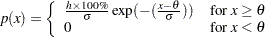
where

threshold parameter
scale parameter
width of histogram interval

The parameter must be less than or equal to the minimum data value. You can specify with the THETA= exponential-option. The default value for is zero. If you specify THETA=EST, a maximum likelihood estimate is computed for . You can specify with the SIGMA= exponential-option. By default, a maximum likelihood estimate is computed for . For example, the following statements fit an exponential curve with and with a maximum likelihood estimate for :

proc capability;
   histogram / exponential(theta=10 l=2 color=red);
run;

The curve is red and has a line type of 2. The EXPONENTIAL option can appear only once in a HISTOGRAM statement. Table 5.18 lists secondary options you can specify with the EXPONENTIAL option. See Formulas for Fitted Curves.

[Traditional Graphics][ODS Graphics] fills areas under a parametric density curve or kernel density estimate with colors and patterns. Enclose the FILL option in parentheses after a curve option or the KERNEL option, as in the following statements:

proc capability;
   histogram length / normal(fill) cfill=green pfill=solid;
run;

Depending on the area to be filled (outside or between the specification limits), you can specify the color and pattern with options in the SPEC statement and HISTOGRAM statement, as summarized in the following table:

If you do not display specification limits, the CFILL= and PFILL= options specify the color and pattern for the entire area under the curve. Solid fills are used by default if patterns are not specified. You can specify the FILL option with only one fitted curve. For an example, see Output 5.8.1. Refer to SAS/GRAPH: Reference for a list of available patterns and colors. If you do not specify the FILL option but specify the options in the preceding table, the colors and patterns are applied to the corresponding areas under the histogram.

forces the creation of a histogram if there is only one unique observation. By default, a histogram is not created if the standard deviation of the data is zero.

[Traditional Graphics] draws reference lines requested with the HREF= and VREF= options in front of the histogram bars. When the NOGSTYLE system option is specified, reference lines are drawn behind the histogram bars by default, and can be obscured by them.

displays a fitted gamma density curve on the histogram. The curve equation is

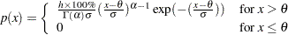
where

threshold parameter
scale parameter
shape parameter
width of histogram interval

The parameter for the gamma distribution must be less than the minimum data value. You can specify with the THETA= gamma-option. The default value for is 0. If you specify THETA=EST, a maximum likelihood estimate is computed for . In addition, the gamma distribution has a shape parameter and a scale parameter . You can specify these parameters with the ALPHA= and SIGMA= gamma-options. By default, maximum likelihood estimates are computed for and . For example, the following statements fit a gamma curve with and with maximum likelihood estimates for and :

proc capability;
   histogram length / gamma(theta=4);
run;

Note that the maximum likelihood estimate of is calculated iteratively using the Newton-Raphson approximation. The ALPHADELTA=, ALPHAINITIAL=, and MAXITER= gamma-options control the approximation.

The GAMMA option can appear only once in a HISTOGRAM statement. Table 5.18 lists secondary options you can specify with the GAMMA option. See Example 5.9 and Formulas for Fitted Curves.

specifies the second shape parameter for Johnson and Johnson density curves requested with the SB and SU options. Enclose the GAMMA= option in parentheses after the SB or SU option. If you do not specify a value for , the procedure calculates an estimate.

[Traditional Graphics][ODS Graphics] adds a grid to the histogram. Grid lines are horizontal lines positioned at major tick marks on the vertical axis.

[Traditional Graphics][Line Printer] requests a hanging histogram , as illustrated in Figure 5.7.6.

data Hang;
   do i=1 to 50;
      Width=14+rannor(34223411)/50;
      output;
   end;
   label Width='Width in cm';
   drop i;
run;

legend2 frame;
title 'Hanging Histogram of Width';
proc capability data=Hang noprint;
   hist / normal(noprint)
          hanging
          legend = legend2
          vref   = 0
          lvref  = 2;
run;

Output 5.7.6 Hanging Histogram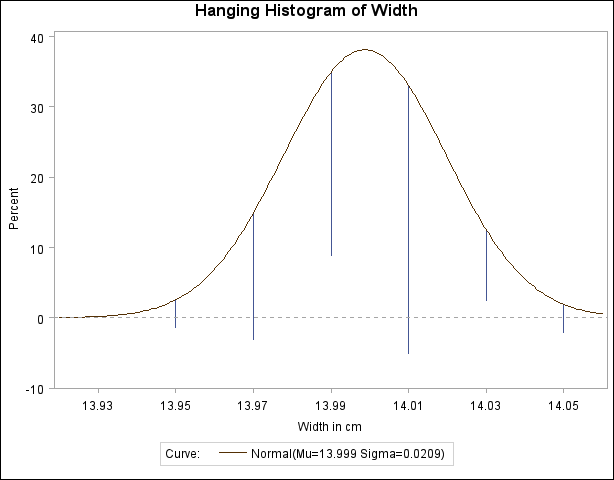

You can use the HANGING option with only one fitted density curve. A hanging histogram aligns the tops of the histogram bars (displayed as lines) with the fitted curve. The lines are positioned at the midpoints of the histogram bins. A hanging histogram is a goodness-of-fit diagnostic in the sense that the closer the lines are to the horizontal axis, the better the fit. Hanging histograms are discussed by Tukey (1977), Wainer (1974), and Velleman and Hoaglin (1981).

[Traditional Graphics] specifies the offset in percent screen units at both ends of the horizontal axis. Specify HOFFSET=0 to eliminate the default offset.

requests capability indices based on the fitted distribution. Enclose the keyword INDICES in parentheses after the distribution keyword. See Indices Using Fitted Curves for computational details and see Output 5.11.2.

[Traditional Graphics] specifies the horizontal space in percent screen units between histogram bars. By default, the bars are contiguous.

specifies the kernel function (normal, quadratic, or triangular) used to compute a kernel density estimate. Enclose the K= option in parentheses after the KERNEL option, as in the following statements:

proc capability;
   histogram length / kernel(k=quadratic);
run;

You can specify kernel functions for up to five estimates. You can also use the K= option together with the C= option, which specifies standardized bandwidths. If you specify more kernel functions than bandwidths, the last bandwidth in the list is repeated for the remaining estimates. Likewise, if you specify more bandwidths than kernel functions, the last kernel function is repeated for the remaining estimates. For example, the following statements compute three estimates with bandwidths of 0.5, 1.0, and 1.5:

proc capability;
   histogram length / kernel(c=0.5 1.0 1.5 k=normal quadratic);
run;

The first estimate uses a normal kernel, and the last two estimates use a quadratic kernel. By default, a normal kernel is used.

superimposes up to five kernel density estimates on the histogram. You can specify the kernel-options described in the following table:

You can request multiple kernel density estimates on the same histogram by specifying a list of values for either the C= or K= option. For more information, see the entries for these options. Also see Output 5.6.1 and Kernel Density Estimates. By default, kernel density estimates are computed using the AMISE method.

[Traditional Graphics] specifies the name of a LEGEND statement describing the legend for specification limit reference lines and fitted curves. Specifying LEGEND=NONE suppresses all legend information and is equivalent to specifying the NOLEGEND option.

[Traditional Graphics] specifies the line type for the grid requested with the GRID option. If you use the LGRID= option, you do not need to specify the GRID option. The default is 1, which produces a solid line.

displays a fitted lognormal density curve on the histogram. The curve equation is

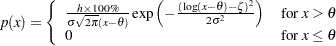
where

threshold parameter
scale parameter
shape parameter
width of histogram interval

Note that the lognormal distribution is also referred to as the distribution in the Johnson system of distributions.

The parameter for the lognormal distribution must be less than the minimum data value. You can specify with the THETA= lognormal-option. The default value for is zero. If you specify THETA=EST, a maximum likelihood estimate is computed for . You can specify the parameters and with the SIGMA= and ZETA= lognormal-options. By default, maximum likelihood estimates are computed for and . For example, the following statements fit a lognormal distribution function with a default value of and with maximum likelihood estimates for and :

proc capability;
   histogram length / lognormal;
run;

The LOGNORMAL option can appear only once in a HISTOGRAM statement. Table 5.18 lists secondary options that you can specify with the LOGNORMAL option. See Example 5.9 and Formulas for Fitted Curves.

specifies lower bounds for kernel density estimates requested with the KERNEL option. Enclose the LOWER= option in parentheses after the KERNEL option. You can specify up to five lower bounds for multiple kernel density estimates. If you specify more kernel estimates than lower bounds, the last lower bound is repeated for the remaining estimates.

specifies the maximum number of bins to be displayed in a comparative histogram. This option is useful in situations where the scales or ranges of the data distributions differ greatly from cell to cell. By default, the bin size and midpoints are determined for the key cell, and then the midpoint list is extended to accommodate the data ranges for the remaining cells. However, if the cell scales differ considerably, the resulting number of bins may be so great that each cell histogram is scaled into a narrow region. By limiting the number of bins with the MAXNBIN= option, you can narrow the window about the data distribution in the key cell. Note that the MAXNBIN= option provides an alternative to the MAXSIGMAS= option.

limits the number of bins to be displayed to a range of value standard deviations (of the data in the key cell) above and below the mean of the data in the key cell. This option is useful in situations where the scales or ranges of the data distributions differ greatly from cell to cell. By default, the bin size and midpoints are determined for the key cell, and then the midpoint list is extended to accommodate the data ranges for the remaining cells. If the cell scales differ considerably, however, the resulting number of bins may be so great that each cell histogram is scaled into a narrow region. By limiting the number of bins with the MAXSIGMAS= option, you narrow the window about the data distribution in the key cell. Note that the MAXSIGMAS= option provides an alternative to the MAXNBIN= option.

requests a table listing the midpoints and percent of observations in each histogram interval. For example, the following statements create the table in Figure 5.7.7:

title;
data Measures;
   input Length @@;
   label Length = 'Attachment Point Offset in mm';
   datalines;
10.147 10.070 10.032 10.042 10.102
10.034 10.143 10.278 10.114 10.127
10.122 10.018 10.271 10.293 10.136
10.240 10.205 10.186 10.186 10.080
10.158 10.114 10.018 10.201 10.065
10.061 10.133 10.153 10.201 10.109
10.122 10.139 10.090 10.136 10.066
10.074 10.175 10.052 10.059 10.077
10.211 10.122 10.031 10.322 10.187
10.094 10.067 10.094 10.051 10.174
;
run;

proc capability;
   histogram Length / midpercents;
run;

If you specify the MIDPERCENTS option in parentheses after a density estimate option, a table listing the midpoints, observed percent of observations, and the estimated percent of the population in each interval (estimated from the fitted distribution) is printed.

The following statements create the table shown in Figure 5.7.8:

proc capability;
   histogram Length / gamma(theta=3 midpercents);
run;

specifies how to determine the midpoints for the histogram intervals, where values-list determines the width of the histogram bars as the difference between consecutive midpoints. The procedure uses the same values for all variables. See Output 5.9.1.

The range of midpoints, extended at each end by half of the bar width, must cover the range of the data as well as any specification limits. For example, if you specify

midpoints=2 to 10 by 0.5

then all of the observations and specification limits should fall between 1.75 and 10.25. (Otherwise, a default list of midpoints is used.) You must use evenly spaced midpoints listed in increasing order.

KEY

determines the midpoints for the data in the key cell. The initial number of midpoints is based on the number of observations in the key cell that use the method of Terrell and Scott (1985). The procedure extends the midpoint list for the key cell in either direction as necessary until it spans the data in the remaining cells.

UNIFORM

determines the midpoints by using all the observations as if there were no cells. In other words, the number of midpoints is based on the total sample size by using the method of Terrell and Scott (1985).

Neither KEY nor UNIFORM apply unless you use the CLASS statement. By default, if you use a CLASS statement, MIDPOINTS=KEY. However, if the key cell is empty then MIDPOINTS=UNIFORM. Otherwise, the procedure computes the midpoints by using the algorithm described in Terrell and Scott (1985). The default midpoints are primarily applicable to continuous data that are approximately normally distributed.

If you produce traditional graphics and use the MIDPOINTS= and HAXIS= options, you can use the ORDER= option in the AXIS statement you specified with the HAXIS= option. However, for the tick mark labels to coincide with the histogram interval midpoints, the range of the ORDER= list must encompass the range of the MIDPOINTS= list, as illustrated in the following statements:

proc capability;
   histogram length / midpoints=20 to 80 by 10
                      haxis=axis1;
   axis1 length=6 in order=10 20 30 40 50 60 70 80 90;
run;

[Traditional Graphics] is an alias for the HAXIS= option described earlier in this section.

specifies the parameter for normal density curves requested with the NORMAL option. Enclose the MU= option in parentheses after the NORMAL option. The default value is the sample mean.

specifies the number of histogram interval endpoints and causes the endpoints, rather than interval midpoints, to be aligned with horizontal axis tick marks.

specifies the number of histogram intervals.

suppresses drawing of histogram bars. This option is useful when you want to display fitted curves only.

suppresses the portion of the legend for fitted curves. If you use the INSET statement to display information about the fitted curve on the histogram, you can use the NOCURVELEGEND option to prevent the information about the fitted curve from being repeated in a legend at the bottom of the histogram. See Output 5.15.1.

suppresses legends for specification limits, fitted curves, distribution lines, and hidden observations. See Example 5.13. Specifying the NOLEGEND option is equivalent to specifying LEGEND=NONE.

suppresses the creation of a plot. Use the NOPLOT option when you want only to print summary statistics for a fitted density or create either an OUTFIT= or an OUTHISTOGRAM= data set. See Example 5.11.

suppresses printed output summarizing the fitted curve. Enclose the NOPRINT option in parentheses following the distribution option. See Customizing a Histogram for an example.

displays a fitted normal density curve on the histogram. The curve equation is

where

mean
standard deviation
width of histogram interval

Note that the normal distribution is also referred to as the distribution in the Johnson system of distributions.

You can specify values for and with the MU= and SIGMA= normal-options, as shown in the following statements:

proc capability;
   histogram length / normal(mu=14 sigma=0.05);
run;

By default, the sample mean and sample standard deviation are used for and . The NORMAL option can appear only once in a HISTOGRAM statement. Table 5.18 lists secondary options that you can specify with the NORMAL option. See Figure 5.7.4 and Formulas for Fitted Curves.

suppresses the portion of the legend for specification limit reference lines. See Figure 5.7.5.

suppresses the table of contents entries for tables produced by the HISTOGRAM statement. See the section ODS Tables for descriptions of the tables produced by the HISTOGRAM statement.

creates a SAS data set that contains parameter estimates for fitted curves and related goodness-of-fit information. See Output Data Sets.

creates a SAS data set that contains information about histogram intervals. Specifically, the data set contains the midpoints of the histogram intervals, the observed percent of observations in each interval, and the estimated percent of observations in each interval (estimated from each of the specified fitted curves). See Output Data Sets.

is an alias for the VAXIS= option.

specifies a list of percents for which quantiles calculated from the data and quantiles estimated from the fitted curve are tabulated. The percents must be between 0 and 100. Enclose the PERCENTS= option in parentheses after the curve option. The default percents are 1, 5, 10, 25, 50, 75, 90, 95, and 99.

For example, the following statements create the table shown in Figure 5.7.9:

proc capability;
   histogram Length / lognormal (percents=1 3 5 95 97 99);
run;

[Traditional Graphics] specifies a pattern used to fill the bars of the histograms (or the areas under a fitted curve if you also specify the FILL option). See the entries for the CFILL= and FILL options for additional details. Refer to SAS/GRAPH: Reference for a list of pattern values. By default, the bars and curve areas are not filled.

includes the right endpoint of each histogram interval in that interval. By default, the left endpoint is included in the histogram interval.

displays a fitted Johnson density curve on the histogram. The curve equation is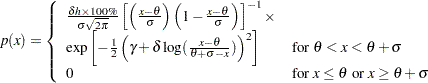

where

threshold parameter
scale parameter
shape parameter
shape parameter
width of histogram interval

The distribution is bounded below by the parameter and above by the value . The parameter must be less than the minimum data value. You can specify with the THETA= -option, or you can request that be estimated with the THETA = EST -option. The default value for is zero. The sum must be greater than the maximum data value. The default value for is one. You can specify with the SIGMA= -option, or you can request that be estimated with the SIGMA = EST -option. You can specify with the DELTA= -option, and you can specify with the GAMMA= -option. Note that the -options are given in parentheses after the SB option.

By default, the method of percentiles is used to estimate the parameters of the distribution. Alternatively, you can request the method of moments or the method of maximum likelihood with the FITMETHOD = MOMENTS or FITMETHOD = MLE options, respectively. Consider the following example:

proc capability;
   histogram length / sb;
   histogram length / sb( theta=est sigma=est );
   histogram length / sb( theta=0.5 sigma=8.4 
                          delta=0.8 gamma=-0.6 );
run;

The first HISTOGRAM statement fits an distribution with default values of and and with percentile-based estimates for and . The second HISTOGRAM statement estimates all four parameters with the method of percentiles. The third HISTOGRAM statement displays an curve with specified values for all four parameters.

The SB option can appear only once in a HISTOGRAM statement. Table 5.18 lists secondary options you can specify with the SB option.

specifies the parameter for curves requested with the BETA, EXPONENTIAL, GAMMA, LOGNORMAL, NORMAL, SB, SU, and WEIBULL options. Enclose the SIGMA= option in parentheses after the distribution option. The following table summarizes the use of the SIGMA= option:

With the BETA distribution option, you can specify SIGMA=EST to request a maximum likelihood estimate for . For syntax examples, see the entries for the BETA and NORMAL options.

specifies the name of a LEGEND statement describing the legend for specification limits and fitted curves. Specifying SPECLEGEND=NONE, which suppresses the portion of the legend for specification limit references lines, is equivalent to specifying the NOSPECLEGEND option.

displays a fitted Johnson density curve on the histogram. The curve equation is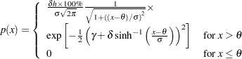

where

location parameter
scale parameter
shape parameter
shape parameter
width of histogram interval

You can specify the parameters with the THETA=, SIGMA=, DELTA=, and GAMMA= -options, which are enclosed in parentheses after the SU option. If you do not specify these parameters, they are estimated.

By default, the method of percentiles is used to estimate the parameters of the distribution. Alternatively, you can request the method of moments or the method of maximum likelihood with the FITMETHOD = MOMENTS or FITMETHOD = MLE options, respectively. Consider the following example:

proc capability;
   histogram length / su;      
   histogram length / su( theta=0.5 sigma=8.4 
                          delta=0.8 gamma=-0.6 );
run;

The first HISTOGRAM statement estimates all four parameters with the method of percentiles. The second HISTOGRAM statement displays an curve with specified values for all four parameters.

The SU option can appear only once in a HISTOGRAM statement. Table 5.18 lists secondary options you can specify with the SU option.

[Line Printer] specifies the character used for the density curve or kernel density curve in line printer plots. Enclose the SYMBOL= option in parentheses after the distribution option or the KERNEL option. The default character is the first letter of the distribution keyword or '1' for the first kernel density estimate, '2' for the second kernel density estimate, and so on. If you use the SYMBOL= option with the KERNEL option, you can specify a list of up to five characters in parentheses for multiple kernel density estimates. If there are more estimates than characters, the last character specified is used for the remaining estimates.

specifies the lower threshold parameter for curves requested with the BETA, EXPONENTIAL, GAMMA, LOGNORMAL, SB, and WEIBULL options, and the location parameter for curves requested with the SU option. Enclose the THETA= option in parentheses after the curve option. See Example 5.8. The default value is zero. If you specify THETA=EST, an estimate is computed for .

is an alias for the THETA= option. See the preceding entry for the THETA= option.

specifies upper bounds for kernel density estimates requested with the KERNEL option. Enclose the UPPER= option in parentheses after the KERNEL option. You can specify up to five upper bounds for multiple kernel density estimates. If you specify more kernel estimates than upper bounds, the last upper bound is repeated for the remaining estimates.

[Traditional Graphics] specifies the offset in percent screen units at the upper end of the vertical axis.

specifies the scale of the vertical axis. The value COUNT scales the data in units of the number of observations per data unit. The value PERCENT scales the data in units of percent of observations per data unit. The value PROPORTION scales the data in units of proportion of observations per data unit. See Figure 5.7.5 for an illustration of VSCALE=COUNT. The default is PERCENT.

[Traditional Graphics] specifies the width of bar outlines. By default, .

displays a fitted Weibull density curve on the histogram. The curve equation is

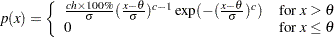
where

threshold parameter
scale parameter
shape parameter
width of histogram interval

The parameter must be less than the minimum data value. You can specify with the THETA= Weibull-option. The default value for is zero. If you specify THETA=EST, a maximum likelihood estimate is computed for . You can specify and with the SIGMA= and C= Weibull-options. By default, maximum likelihood estimates are computed for and . For example, the following statements fit a Weibull distribution with and with maximum likelihood estimates for and :

proc capability;
   histogram length / weibull(theta=15);
run;

Note that the maximum likelihood estimate of is calculated iteratively using the Newton-Raphson approximation. The CDELTA=, CINITIAL=, and MAXITER= Weibull-options control the approximation.

The WEIBULL option can appear only once in a HISTOGRAM statement. Table 5.18 lists secondary options that you can specify with the WEIBULL option. See Example 5.9 and Formulas for Fitted Curves.

[Traditional Graphics] specifies the width of the grid lines requested with the GRID option. By default, grid lines are the same width as the axes. If you use the WGRID= option, you do not need to specify the GRID option.

specifies a value for the scale parameter for lognormal density curves requested with the LOGNORMAL option. Enclose the ZETA= option in parentheses after the LOGNORMAL option. By default, the procedure calculates a maximum likelihood estimate for . You can specify the SCALE= option as an alias for the ZETA= option.