The HPBIN Procedure

Quantile binning requires data to be sorted in a particular way, and the sorting process usually consumes a significant amount of CPU time and memory size. When the input data set is larger than the available memory, the sorting algorithm becomes more complicated. In distributed computing, data communications overhead also increases the sorting challenge.

To address these issues, the HPBIN procedure offers a novel approach to quantile binning, called pseudo–quantile binning. The pseudo–quantile binning method is very efficient, and the results mimic those of the quantile binning method. For example, consider the following statements:

    data bindata;
        do i=1 to 1000;
    	    x=rannorm(1);
    	    output;
        end;
    run;

 proc rank data=bindata out=rankout group=8;
     var x;
     ranks rank_x;
 run;

 proc univariate data=rankout plot;
     var rank_x;
     histogram;
 run;

These statements create a data set that contains 1,000 observations, each generated from a random normal distribution. The histogram for this data set is shown in Figure 4.1.

The pseudo–quantile binning method in the HPBIN procedure can achieve a similar result by using far less computation time. In this case, the time complexity is , where is a constant and is the number of observations. When the algorithm runs on the grid, the total amount of computation time is much less. For example, if a cluster has 32 nodes and each node has 24 shared-memory CPUs, then the time complexity is .

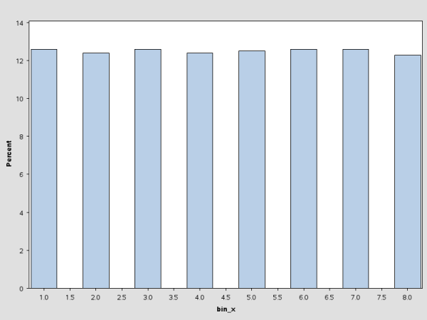
The following statements bin the data by using the PSEUDO_QUANTILE option in the PROC HPBIN statement and generate the histogram for the binning output data. (See Figure 4.2.) This histogram is similar to the one in Figure 4.1.

 proc hpbin data=bindata output=binout numbin=8 pseudo_quantile;
     input x;
 run;

 proc univariate data=binout plot;
     var bin_x;
     histogram;
 run;