| Selected Examples |
Nonhomogeneous Poisson Processes
In many situations, the arrival rate or service rate is determined by a Poisson process whose parameter varies as a function of time. For example, if the arrival rate to a fast food restaurant varies with the time of day and increases to a local maximum during meal times, you can sample from a nonhomogeneous Poisson process. In the QSIM Application, there are some limitations to the shape of the rate function that are allowed. This function must be cyclical and bounded. The software takes the absolute value of the rate function to guarantee that it is nonnegative.
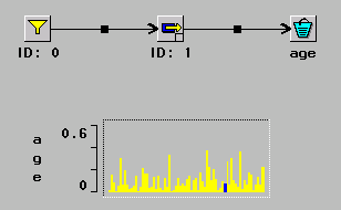
In this example, shown in Figure 10.9,
the model has deterministic arrival rate and nonhomogeneous
Poisson service times.

|
Figure 10.9: Nonhomogeneous Poisson Service
The service rate is ![]() , where
, where ![]() is the
value of the simulation time when a sample is taken.
This rate function is specified via the control panel for the
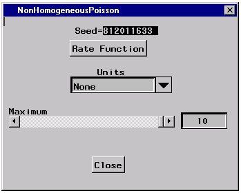
random variable, as shown in Figure 10.10.
is the
value of the simulation time when a sample is taken.
This rate function is specified via the control panel for the
random variable, as shown in Figure 10.10.

|
Figure 10.10: Nonhomogeneous Poisson Control Panel
In this window you can set two parameters of the process: the
rate function and the maximum value that the rate function can
take.
The rate function is specified as a QSIM formula.
When you click
the Rate Function button, a Formula Manager window
opens and allows you to specify the function.
|
|
Figure 10.11: Rate Function
Figure 10.11 shows the function used in this example.
The maximum is needed by the algorithm that does the sampling.
If this is not the correct maximum or the function specified
is not cyclical, then the sample is not from the desired
distribution.
When the transactions from this simple model are displayed in the LinePlot as shown in Figure 10.9, you can see the impact of the cyclical rate function on the transaction time in the system.
Copyright © 2008 by SAS Institute Inc., Cary, NC, USA. All rights reserved.