The Earned Value Management Macros

Example 11.1 Integrated Assembly Project
The planned schedule for an assembly project is shown in Output 11.1.1. This schedule can be computed by either of the CPM or PM procedures. (For more details, see Chapter 4 or Chapter 5, respectively.)
Output 11.1.1: Schedule IOUT1
| Integrated Assembly Test Project |
| Initial Schedule |
| Obs | Activity | Duration | Description | Planned Start | Planned Finish |
|---|---|---|---|---|---|
| 1 | S | 0 | Start | 01OCT09 | 01OCT09 |
| 2 | PD | 105 | Preliminary Design | 01OCT09 | 13JAN10 |
| 3 | PDR | 21 | Prelim Design Review | 14JAN10 | 03FEB10 |
| 4 | FD | 168 | Final Design | 04FEB10 | 21JUL10 |
| 5 | PM | 126 | Procure Material | 10JUN10 | 13OCT10 |
| 6 | FDR | 21 | Final Design Review | 22JUL10 | 11AUG10 |
| 7 | FP | 273 | Facility Preparation | 01OCT10 | 30JUN11 |
| 8 | FC | 273 | Fabricate Components | 12AUG10 | 11MAY11 |
| 9 | DA | 26 | Deliver Assembly | 26JUN11 | 21JUL11 |
| 10 | FRR | 21 | Facil Readiness Rvw | 01JUL11 | 21JUL11 |
| 11 | IA | 42 | Install Assembly | 22JUL11 | 01SEP11 |
| 12 | RR | 21 | Readiness Review | 02SEP11 | 22SEP11 |
| 13 | T | 126 | Test | 01OCT11 | 03FEB12 |
| 14 | TV | 63 | Test Validation | 07JAN12 | 09MAR12 |
The budgeted cost rates are given in Output 11.1.2. It is assumed that the activities incur costs continuously.
Output 11.1.2: Cost Rates IATCOST
The budgeted periodic cost can now be generated with the following specification of the %EVA_PLANNED_VALUE macro:
%eva_planned_value(
    plansched=iout1,
    activity=activity,
    start=start,
    finish=finish,
    duration=duration,
    budgetcost=iatcost,
    rate=rate
);
For brevity, only the first 17 rows of the output data set are shown in Output 11.1.3.
Output 11.1.3: %EVA_PLANNED_VALUE: Periodic Data Set
| Daily Planned Value |
| Obs | Period Identifier | PV Rate |
|---|---|---|
| 1 | 01OCT09 | 4.76190 |
| 2 | 02OCT09 | 4.76190 |
| 3 | 03OCT09 | 4.76190 |
| 4 | 04OCT09 | 4.76190 |
| 5 | 05OCT09 | 4.76190 |
| 6 | 06OCT09 | 4.76190 |
| 7 | 07OCT09 | 4.76190 |
| 8 | 08OCT09 | 4.76190 |
| 9 | 09OCT09 | 4.76190 |
| 10 | 10OCT09 | 4.76190 |
| 11 | 11OCT09 | 4.76190 |
| 12 | 12OCT09 | 4.76190 |
| 13 | 13OCT09 | 4.76190 |
| 14 | 14OCT09 | 4.76190 |
| 15 | 15OCT09 | 4.76190 |
| 16 | 16OCT09 | 4.76190 |
| 17 | 17OCT09 | 4.76190 |
Next, the actual progress of the project through September 30, 2010, is entered. The ACTUAL data set is shown in Output 11.1.4.
Output 11.1.4: Current Status ACTUAL
These inputs are then used by the CPM procedure with the original schedule to produce an updated schedule, given in Output 11.1.5. (For information about using the CPM procedure, see Chapter 4.)
Output 11.1.5: Updated Schedule UPDSCHED
| Updated Schedule |
| Obs | Activity | Actual Duration | Description | Pct. Comp. | Start | Finish |
|---|---|---|---|---|---|---|
| 1 | S | 0 | Start | 100 | 01OCT09 | 01OCT09 |
| 2 | PD | 121 | Preliminary Design | 100 | 01OCT09 | 29JAN10 |
| 3 | PDR | 21 | Prelim Design Review | 100 | 30JAN10 | 19FEB10 |
| 4 | FD | 203 | Final Design | 100 | 20FEB10 | 10SEP10 |
| 5 | PM | . | Procure Material | 40 | 10AUG10 | 17DEC10 |
| 6 | FDR | . | Final Design Review | 80 | 11SEP10 | 05OCT10 |
| 7 | FP | . | Facility Preparation | . | 06OCT10 | 05JUL11 |
| 8 | FC | . | Fabricate Components | . | 12OCT10 | 11JUL11 |
| 9 | DA | . | Deliver Assembly | . | 07JUL11 | 01AUG11 |
| 10 | FRR | . | Facil Readiness Rvw | . | 06JUL11 | 26JUL11 |
| 11 | IA | . | Install Assembly | . | 02AUG11 | 12SEP11 |
| 12 | RR | . | Readiness Review | . | 13SEP11 | 03OCT11 |
| 13 | T | . | Test | . | 04OCT11 | 06FEB12 |
| 14 | TV | . | Test Validation | . | 10JAN12 | 12MAR12 |
The %EVA_EARNED_VALUE macro can then be used to generate the updated periodic cost, as follows:
%eva_earned_value(
    revisesched=updsched,
    activity=activity,
    start=start,
    finish=finish,
    actualcost=iatupd,
    rate=rate
);
Again, for brevity only the first 17 rows of the output data set are shown in Output 11.1.6.
Output 11.1.6: %EVA_EARNED_VALUE: Periodic Data Set
| Daily Earned Value and Revised Cost |
| Obs | Period Identifier | EV Rate | AC Rate |
|---|---|---|---|
| 1 | 01OCT09 | 4.13223 | 6 |
| 2 | 02OCT09 | 4.13223 | 6 |
| 3 | 03OCT09 | 4.13223 | 6 |
| 4 | 04OCT09 | 4.13223 | 6 |
| 5 | 05OCT09 | 4.13223 | 6 |
| 6 | 06OCT09 | 4.13223 | 6 |
| 7 | 07OCT09 | 4.13223 | 6 |
| 8 | 08OCT09 | 4.13223 | 6 |
| 9 | 09OCT09 | 4.13223 | 6 |
| 10 | 10OCT09 | 4.13223 | 6 |
| 11 | 11OCT09 | 4.13223 | 6 |
| 12 | 12OCT09 | 4.13223 | 6 |
| 13 | 13OCT09 | 4.13223 | 6 |
| 14 | 14OCT09 | 4.13223 | 6 |
| 15 | 15OCT09 | 4.13223 | 6 |
| 16 | 16OCT09 | 4.13223 | 6 |
| 17 | 17OCT09 | 4.13223 | 6 |
The %EVA_METRICS macro can be called with a current date of September 30, 2010, as follows:
%eva_metrics(
    timenow='30sep10'd,
    acronyms=long
);
Output 11.1.7 shows the output listing from %EVA_METRICS. Notice that "ACRONYMS=long" is specified, which results in the long version of the earned value acronyms being used.
Output 11.1.7: %EVA_METRICS: Summary Statistics
| Earned Value Analysis |
| as of September 30, 2010 |
| Metric | Value |
|---|---|
| Percent Complete | 20.66 |
| BCWS (Budgeted Cost of Work Scheduled) | 2038.00 |
| BCWP (Budgeted Cost of Work Performed) | 1374.00 |
| ACWP (Actual Cost of Work Performed) | 2020.30 |
| CV (Cost Variance) | -646.30 |
| CV% | -47.04 |
| SV (Schedule Variance) | -664.00 |
| SV% | -32.58 |
| CPI (Cost Performance Index) | 0.68 |
| SPI (Schedule Performance Index) | 0.67 |
| BAC (Budget At Completion) | 6650.00 |
| EAC (Revised Estimate At Completion) | 7349.50 |
| EAC (Overrun to Date) | 7296.30 |
| EAC (Cumulative CPI) | 9778.02 |
| EAC (Cumulative CPI X SPI) | 13527.00 |
| ETC (Estimate To Complete)* | 7757.72 |
| VAC (Variance At Completion)* | -3128.02 |
| VAC%* | -47.04 |
| TCPI (BAC) (To-Complete Performance Index) | 1.14 |
| TCPI (EAC) (To-Complete Performance Index)* | 0.68 |
| * The CPI form of the EAC is used. |
Next, the %EVA_TASK_METRICS macro is used to produce Cost and Schedule Variance by task.
%eva_task_metrics(
    plansched=iout1,
    revisesched=updsched,
    activity=activity,
    start=start,
    finish=finish,
    pctcomp=pctcomp,
    budgetcost=iatcost,
    actualcost=iatupd,
    rate=rate,
    timenow='30sep10'd,
    acronyms=long
);
The output listing is shown in Output 11.1.8.
Output 11.1.8: %EVA_TASK_METRICS: CV and SV by Activity
| Earned Value Analysis by Activity |
| as of September 30, 2010 |
| Obs | Activity | BCWS | BCWP | ACWP | CV | CV% | SV | SV% | CPI | SPI |
|---|---|---|---|---|---|---|---|---|---|---|
| 1 | S | 0.00 | 0.00 | 0.00 | 0.00 | 0.00 | 0.00 | 0.00 | . | . |
| 2 | PD | 500.00 | 500.00 | 726.00 | -226.00 | -45.20 | 0.00 | 0.00 | 0.69 | 1.00 |
| 3 | PDR | 150.00 | 150.00 | 172.20 | -22.20 | -14.80 | 0.00 | 0.00 | 0.87 | 1.00 |
| 4 | FD | 300.00 | 300.00 | 629.30 | -329.30 | -109.77 | 0.00 | 0.00 | 0.48 | 1.00 |
| 5 | PM | 681.59 | 304.00 | 332.80 | -28.80 | -9.47 | -377.59 | -55.40 | 0.91 | 0.45 |
| 6 | FDR | 150.00 | 120.00 | 160.00 | -40.00 | -33.33 | -30.00 | -20.00 | 0.75 | 0.80 |
| 7 | FP | 0.00 | 0.00 | 0.00 | 0.00 | 0.00 | 0.00 | 0.00 | . | . |
| 8 | FC | 256.41 | 0.00 | 0.00 | 0.00 | 0.00 | -256.41 | -100.00 | . | 0.00 |
| 9 | DA | 0.00 | 0.00 | 0.00 | 0.00 | 0.00 | 0.00 | 0.00 | . | . |
| 10 | FRR | 0.00 | 0.00 | 0.00 | 0.00 | 0.00 | 0.00 | 0.00 | . | . |
| 11 | IA | 0.00 | 0.00 | 0.00 | 0.00 | 0.00 | 0.00 | 0.00 | . | . |
| 12 | RR | 0.00 | 0.00 | 0.00 | 0.00 | 0.00 | 0.00 | 0.00 | . | . |
| 13 | T | 0.00 | 0.00 | 0.00 | 0.00 | 0.00 | 0.00 | 0.00 | . | . |
| 14 | TV | 0.00 | 0.00 | 0.00 | 0.00 | 0.00 | 0.00 | 0.00 | . | . |
Output 11.1.9 through Output 11.1.13 show charts that are produced using the earned value analysis reporting macros. First, the %EVG_COST_PLOT macro is used to generate the plot in Output 11.1.9.
%evg_cost_plot(acronyms=long);
Output 11.1.9: %EVG_COST_PLOT, EV, PV, AC, and EAC
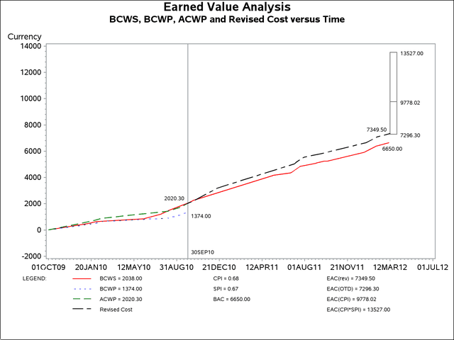
According to the plan, the earned value percentage complete at the status date of September 30, 2010 (shown by the BCWS plot) should have been 2049/6650, or 30.81%. Instead, the percentage complete (shown by the BCWP plot) is only 1374/6650, or 20.66%.
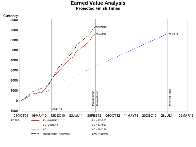
Next, the %EVG_SCHEDULE_PLOT macro is used to produce the plot in Output 11.1.10. The resulting output shows a disastrous projected completion date of August 1, 2014, based upon the current earned value.
This is two years and four months behind the planned schedule end date of March 10, 2012. Based on the performance of the
project so far, it is estimated to cost $9793 at completion (EAC ), amounting to nearly a 50% overrun.
%evg_schedule_plot;
Output 11.1.10: %EVG_SCHEDULE_PLOT: Projected Completion Date
The %EVG_INDEX_PLOT macro is then used to produce the plot in Output 11.1.11.
%evg_index_plot;
Output 11.1.11: %EVG_INDEX_PLOT: Cost and Schedule Performance Index
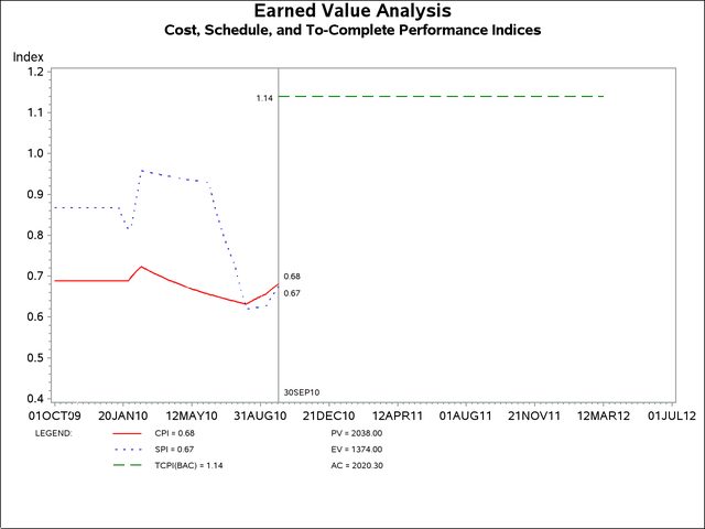
The plot in Output 11.1.11 shows that the performance factor must be increased from 0.68 to 1.14 in order to stay within the budget.
The %EVG_VARIANCE_PLOT macro is used to produce the plot in Output 11.1.12.
%evg_variance_plot;
Output 11.1.12: %EVG_VARIANCE_PLOT: Cost and Schedule Variance
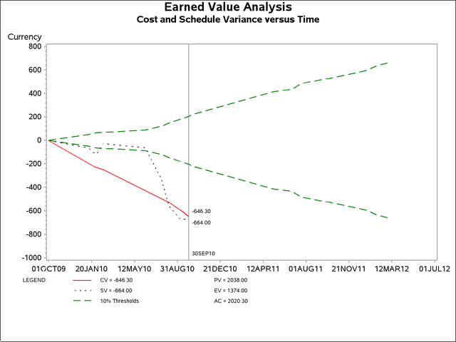
The plot in Output 11.1.12 shows that both the cost and schedule variance have strayed outside of the area between the 10% threshold plots of the planned value.
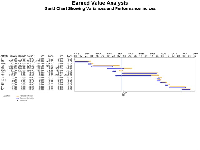
Finally, the %EVG_GANTT_CHART macro is used to produce the Gantt chart shown in Output 11.1.13.
%evg_gantt_chart(
    plansched=iout1,
    revisesched=updsched,
    activity=activity,
    start=start,
    finish=finish,
    duration=duration,
    timenow='30sep10'd,
    id=pv ev ac cv cvp sv svp,
    height=3,
    scale=1.5
);
Output 11.1.13: %EVG_GANTT_CHART: Cost and Schedule Variance by Task