The Earned Value Management Macros

Example 9.1: Integrated Assembly Project

The planned schedule for an assembly project is shown in Figure 9.1.1. This schedule can be computed by either of the CPM or PM procedures. (For more details, see SAS/OR User's Guide: Project Management, Chapter 2 or Chapter 6, respectively.)

Output 9.1.1: Schedule IOUT1

Integrated Assembly Test Project Initial Schedule Obs Activity Duration Description Planned Start Planned Finish 1 S 0 Start 01OCT03 01OCT03 2 PD 105 Preliminary Design 01OCT03 13JAN04 3 PDR 21 Prelim Design Review 14JAN04 03FEB04 4 FD 168 Final Design 04FEB04 20JUL04 5 PM 126 Procure Material 09JUN04 12OCT04 6 FDR 21 Final Design Review 21JUL04 10AUG04 7 FP 273 Facility Preparation 01OCT04 30JUN05 8 FC 273 Fabricate Components 11AUG04 10MAY05 9 DA 26 Deliver Assembly 26JUN05 21JUL05 10 FRR 21 Facil Readiness Rvw 01JUL05 21JUL05 11 IA 42 Install Assembly 22JUL05 01SEP05 12 RR 21 Readiness Review 02SEP05 22SEP05 13 T 126 Test 01OCT05 03FEB06 14 TV 63 Test Validation 07JAN06 10MAR06

The budgeted cost rates are given in Figure 9.1.2. It is assumed that the activities incur costs continuously.

Output 9.1.2: Cost Rates IATCOST

Budgeted Costs Obs Activity Rate 1 S 0.0000 2 PD 4.7619 3 PDR 7.1429 4 FD 1.7857 5 PM 6.0317 6 FDR 7.1429 7 FP 4.0293 8 FC 5.1282 9 DA 13.0769 10 FRR 7.1429 11 IA 5.9524 12 RR 7.1429 13 T 7.1429 14 TV 7.9365

The budgeted periodic cost can now be generated with the following specification of the %EVA_PLANNED_VALUE macro:

    %eva_planned_value(
        plansched=iout1,
        activity=activity,
        start=start,
        finish=finish,
        duration=duration,
        budgetcost=iatcost,
        rate=rate
    );
 

For brevity, only the first 17 rows of the output data set are shown in Figure 9.1.3.

Output 9.1.3: %EVA_PLANNED_VALUE: Periodic Data Set

Daily Planned Value Obs Period Identifier PV Rate 1 01OCT03 4.76190 2 02OCT03 4.76190 3 03OCT03 4.76190 4 04OCT03 4.76190 5 05OCT03 4.76190 6 06OCT03 4.76190 7 07OCT03 4.76190 8 08OCT03 4.76190 9 09OCT03 4.76190 10 10OCT03 4.76190 11 11OCT03 4.76190 12 12OCT03 4.76190 13 13OCT03 4.76190 14 14OCT03 4.76190 15 15OCT03 4.76190 16 16OCT03 4.76190 17 17OCT03 4.76190

Next, the actual progress of the project through September 30, 2004, is entered. The ACTUAL data set is shown in Figure 9.1.4.

Output 9.1.4: Current Status ACTUAL

Status Obs Activity Actual Start Actual Finish Actual Rate Pct. Comp. 1 S 01OCT03 01OCT03 0.0 100 2 PD 01OCT03 29JAN04 6.0 100 3 PDR 30JAN04 19FEB04 8.2 100 4 FD 20FEB04 10SEP04 3.1 100 5 PM 10AUG04 . 6.4 40 6 FDR 11SEP04 . 8.0 80

These inputs are then used by the CPM procedure with the original schedule to produce an updated schedule, given in Figure 9.1.5. (For information on using the CPM procedure, see SAS/OR User's Guide: Project Management, Chapter 2.)

Output 9.1.5: Updated Schedule UPDSCHED

Updated Schedule Obs Activity Actual Duration Description Pct. Comp. Start Finish 1 S 0 Start 100 01OCT03 01OCT03 2 PD 121 Preliminary Design 100 01OCT03 29JAN04 3 PDR 21 Prelim Design Review 100 30JAN04 19FEB04 4 FD 204 Final Design 100 20FEB04 10SEP04 5 PM . Procure Material 40 10AUG04 17DEC04 6 FDR . Final Design Review 80 11SEP04 05OCT04 7 FP . Facility Preparation . 06OCT04 05JUL05 8 FC . Fabricate Components . 12OCT04 11JUL05 9 DA . Deliver Assembly . 07JUL05 01AUG05 10 FRR . Facil Readiness Rvw . 06JUL05 26JUL05 11 IA . Install Assembly . 02AUG05 12SEP05 12 RR . Readiness Review . 13SEP05 03OCT05 13 T . Test . 04OCT05 06FEB06 14 TV . Test Validation . 10JAN06 13MAR06

The %EVA_EARNED_VALUE macro can then be used to generate the updated periodic cost, as follows:

    %eva_earned_value(
        revisesched=updsched,
        activity=activity,
        start=start,
        finish=finish,
        actualcost=iatupd,
        rate=rate
    );
 

Again, for brevity only the first 17 rows of the output data set are shown in Figure 9.1.6.

Output 9.1.6: %EVA_EARNED_VALUE: Periodic Data Set

Daily Earned Value and Revised Cost Obs Period Identifier EV Rate AC Rate 1 01OCT03 4.13223 6 2 02OCT03 4.13223 6 3 03OCT03 4.13223 6 4 04OCT03 4.13223 6 5 05OCT03 4.13223 6 6 06OCT03 4.13223 6 7 07OCT03 4.13223 6 8 08OCT03 4.13223 6 9 09OCT03 4.13223 6 10 10OCT03 4.13223 6 11 11OCT03 4.13223 6 12 12OCT03 4.13223 6 13 13OCT03 4.13223 6 14 14OCT03 4.13223 6 15 15OCT03 4.13223 6 16 16OCT03 4.13223 6 17 17OCT03 4.13223 6

The %EVA_METRICS macro can be called with a current date of September 30, 2004, as follows:

    %eva_metrics(
        timenow='30sep04'd,
        acronyms=long
    );
 

Figure 9.1.7 shows the output listing from %EVA_METRICS. Notice that "ACRONYMS=long" is specified, which results in the long version of the earned value acronyms being used.

Output 9.1.7: %EVA_METRICS: Summary Statistics

Earned Value Analysis as of September 30, 2004 Metric Value Percent Complete 20.66 BCWS (Budgeted Cost of Work Scheduled) 2049.16 BCWP (Budgeted Cost of Work Performed) 1374.00 ACWP (Actual Cost of Work Performed) 2023.40 CV (Cost Variance) -649.40 CV% -47.26 SV (Schedule Variance) -675.16 SV% -32.95 CPI (Cost Performance Index) 0.68 SPI (Schedule Performance Index) 0.67 BAC (Budget At Completion) 6650.00 EAC (Revised Estimate At Completion) 7352.60 EAC (Overrun to Date) 7299.40 EAC (Cumulative CPI) 9793.02 EAC (Cumulative CPI X SPI) 13610.86 ETC (Estimate To Complete)* 7769.62 VAC (Variance At Completion)* -3143.02 VAC%* -47.26 TCPI (BAC) (To-Complete Performance Index) 1.14 TCPI (EAC) (To-Complete Performance Index)* 0.68 * The CPI form of the EAC is used.

Next, the %EVA_TASK_METRICS macro is used to produce Cost and Schedule Variance by task.

    %eva_task_metrics(
     plansched=iout1,
     revisesched=updsched,
     activity=activity,
     start=start,
     finish=finish,
     pctcomp=pctcomp,
     budgetcost=iatcost,
     actualcost=iatupd,
     rate=rate,
     timenow='30sep04'd,
     acronyms=long
    );
 

The output listing is shown in Figure 9.1.8.

Output 9.1.8: %EVA_TASK_METRICS: CV and SV by Activity

Earned Value Analysis by Activity as of September 30, 2004 Obs Activity BCWS BCWP ACWP CV CV% SV SV% CPI SPI 1 S 0.00 0.00 0.00 0.00 0.00 0.00 0.00 . . 2 PD 500.00 500.00 726.00 -226.00 -45.20 0.00 0.00 0.69 1.00 3 PDR 150.00 150.00 172.20 -22.20 -14.80 0.00 0.00 0.87 1.00 4 FD 300.00 300.00 632.40 -332.40 -110.80 0.00 0.00 0.47 1.00 5 PM 687.62 304.00 332.80 -28.80 -9.47 -383.62 -55.79 0.91 0.44 6 FDR 150.00 120.00 160.00 -40.00 -33.33 -30.00 -20.00 0.75 0.80 7 FP 0.00 0.00 0.00 0.00 0.00 0.00 0.00 . . 8 FC 261.54 0.00 0.00 0.00 0.00 -261.54 -100.00 . 0.00 9 DA 0.00 0.00 0.00 0.00 0.00 0.00 0.00 . . 10 FRR 0.00 0.00 0.00 0.00 0.00 0.00 0.00 . . 11 IA 0.00 0.00 0.00 0.00 0.00 0.00 0.00 . . 12 RR 0.00 0.00 0.00 0.00 0.00 0.00 0.00 . . 13 T 0.00 0.00 0.00 0.00 0.00 0.00 0.00 . . 14 TV 0.00 0.00 0.00 0.00 0.00 0.00 0.00 . .

Figure 9.1.9 through Figure 9.1.13 show charts that are produced using the earned value analysis reporting macros. First, the %EVG_COST_PLOT macro is used to generate the plot in Figure 9.1.9.

    %evg_cost_plot(acronyms=long);
 

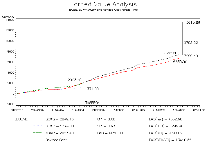
Output 9.1.9: %EVG_COST_PLOT,EV,PV,AC,and EAC

According to the plan, the earned value percentage complete at the status date of September 30, 2004 (shown by the BCWS plot) should have been 2049/6650, or 30.81%. Instead, the percentage complete (shown by the BCWP plot) is only 1374/6650, or 20.66%.

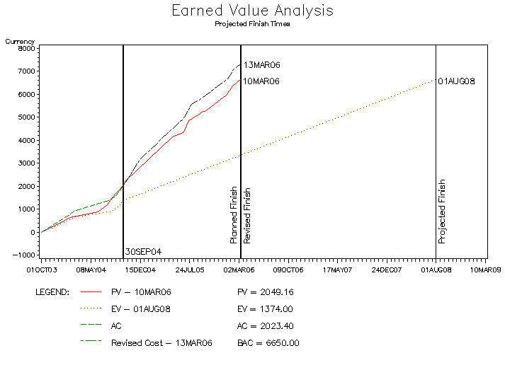
Next, the %EVG_SCHEDULE_PLOT macro is used to produce the plot in Figure 9.1.10. The resulting output shows a disastrous projected completion date of August 1, 2008, based upon the current earned value. This is two years and four months behind the planned schedule end date of March 10, 2006. Based on the performance of the project so far, it is estimated to cost $9793 at completion (EAC), amounting to nearly a 50% overrun.

    %evg_schedule_plot;
 

Output 9.1.10: %EVG_SCHEDULE_PLOT: Projected Completion Date

The %EVG_INDEX_PLOT macro is then used to produce the plot in Figure 9.1.11.

    %evg_index_plot;
 

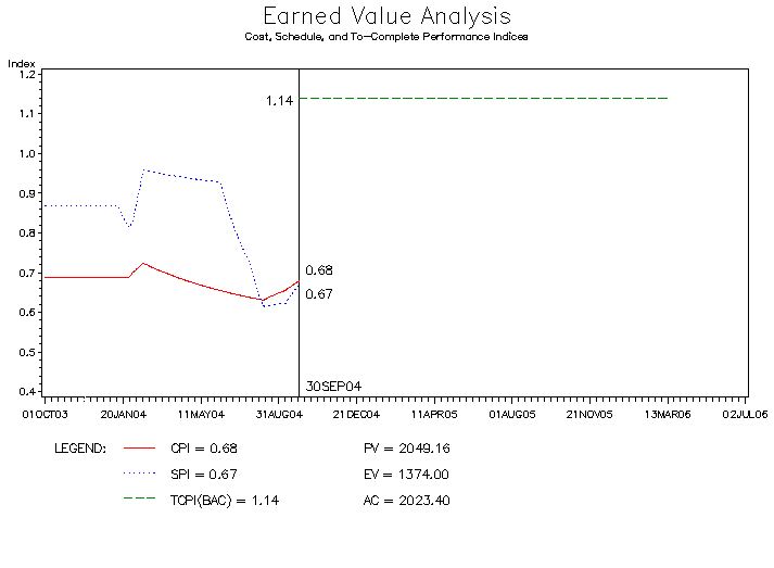
Output 9.1.11: %EVG_INDEX_PLOT: Cost and Schedule Performance Index

The plot in Figure 9.1.11 shows that the performance factor must be increased from 0.68 to 1.14 in order to stay within the budget.

The %EVG_VARIANCE_PLOT macro is used to produce the plot in Figure 9.1.12.

    %evg_variance_plot;
 

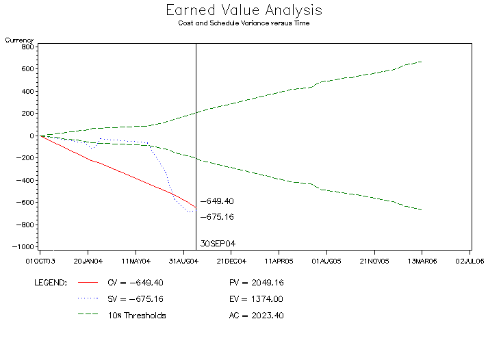
Output 9.1.12: %EVG_VARIANCE_PLOT: Cost and Schedule Variance

The plot in Figure 9.1.12 shows that both the cost and schedule variance have strayed outside of the area between the 10% threshold plots of the planned value.

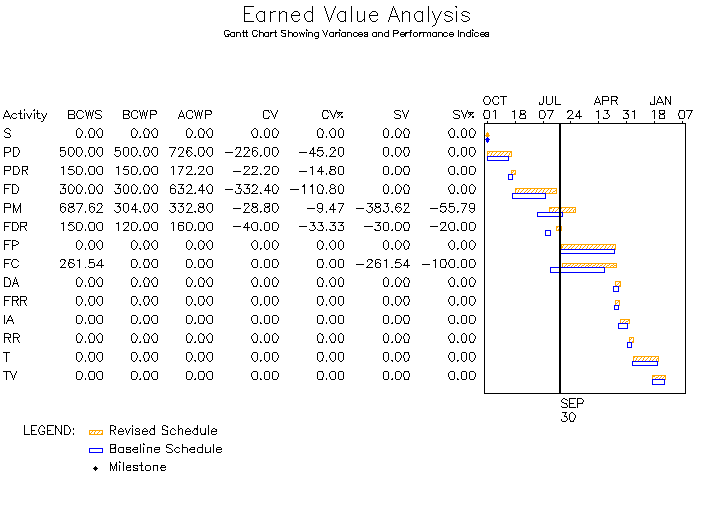
Finally, the %EVG_GANTT_CHART macro is used to produce the Gantt chart shown in Figure 9.1.13.

    %evg_gantt_chart(
        plansched=iout1,
        revisesched=updsched,
        activity=activity,
        start=start,
        finish=finish,
        duration=duration,
        timenow='30sep04'd,
        id=pv ev ac cv cvp sv svp,
        height=3,
        scale=0.5
    );
 

Output 9.1.13: %EVG_GANTT_CHART: Cost and Schedule Variance by Task