The OPTQP Procedure

Overview: OPTQP Procedure
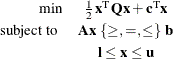
The OPTQP procedure solves quadratic programs—problems with quadratic objective function and a collection of linear constraints, including lower or upper bounds (or both) on the decision variables.
Mathematically, a quadratic programming (QP) problem can be stated as follows:
where
|
|
|
|
is the quadratic (also known as Hessian) matrix |
|
|
|
|
is the constraints matrix |
|
|
|
|
is the vector of decision variables |
|
|
|
|
is the vector of linear objective function coefficients |
|
|
|
|
is the vector of constraints right-hand sides (RHS) |
|
|
|
|
is the vector of lower bounds on the decision variables |
|
|
|
|
is the vector of upper bounds on the decision variables |


The quadratic matrix  is assumed to be symmetric; that is,
![\[ q_{ij} = q_{ji},\quad \forall i,j = 1, \ldots , n \]](images/ormpug_optqp0014.png)
Indeed, it is easy to show that even if  , the simple modification
![\[ \tilde{\mathbf{Q}} = \frac{1}{2}(\mathbf{Q} + \mathbf{Q}^\textrm {T}) \]](images/ormpug_optqp0016.png)
produces an equivalent formulation  hence symmetry is assumed. When you specify a quadratic matrix, it suffices to list only lower triangular coefficients.
In addition to being symmetric, is also required to be positive semidefinite,
![\[ \mathbf{x}^\textrm {T}\mathbf{Qx} \ge 0,\quad \forall \mathbf{x}\in \mathbb {R}^ n \]](images/ormpug_optqp0018.png)
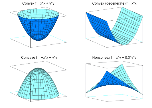
for minimization type of models; it is required to be negative semidefinite for the maximization type of models. Convexity can come as a result of a matrix-matrix multiplication
![\[ \mathbf{Q} = \mathbf{L}\mathbf{L}^\textrm {T} \]](images/ormpug_optqp0019.png)
or as a consequence of physical laws, and so on. See Figure 14.1 for examples of convex, concave, and nonconvex objective functions.
Figure 14.1: Examples of Convex, Concave, and Nonconvex Objective Functions
The order of constraints is insignificant. Some or all components of  or
or  (lower and upper bounds, respectively) can be omitted.