The Quadratic Programming Solver

Example 8.2 Portfolio Optimization
Consider a portfolio optimization example. The two competing goals of investment are (1) long-term growth of capital and (2) low risk. A good portfolio grows steadily without wild fluctuations in value. The Markowitz model is an optimization model for balancing the return and risk of a portfolio. The decision variables are the amounts invested in each asset. The objective is to minimize the variance of the portfolio’s total return, subject to the constraints that (1) the expected growth of the portfolio reaches at least some target level and (2) you do not invest more capital than you have.
Let  be the amount invested in each asset,
  be the amount of capital you have,
  be the random vector of asset returns over some period, and
  be the expected value of . Let
  be the minimum growth you hope to obtain, and
  be the covariance matrix of . The objective function is
  , which can be equivalently denoted as
  .
.
Assume, for example,  = 4. Let = 10,000, = 1,000,
 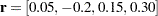 , and
, and
 |
The QP formulation can be written as:
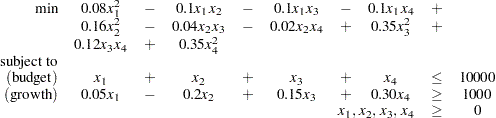 |
Use the following SAS statements to solve the problem:
/* example 2: portfolio optimization */
proc optmodel;
   /* let x1, x2, x3, x4 be the amount invested in each asset */
   var x{1..4} >= 0;

   num coeff{1..4, 1..4} = [0.08 -.05 -.05 -.05
                            -.05 0.16 -.02 -.02
                            -.05 -.02 0.35 0.06
                            -.05 -.02 0.06 0.35];
   num r{1..4}=[0.05 -.20 0.15 0.30];

   /* minimize the variance of the portfolio's total return */
   minimize f = sum{i in 1..4, j in 1..4}coeff[i,j]*x[i]*x[j];

   /* subject to the following constraints */
   con BUDGET: sum{i in 1..4}x[i] <= 10000;
   con GROWTH: sum{i in 1..4}r[i]*x[i] >= 1000;

   solve with qp;

   /* print the optimal solution */
   print x;
The summaries and the optimal solution are shown in Output 8.2.1.
| Problem Summary | |
|---|---|
| Objective Sense | Minimization |
| Objective Function | f |
| Objective Type | Quadratic |
| Number of Variables | 4 |
| Bounded Above | 0 |
| Bounded Below | 4 |
| Bounded Below and Above | 0 |
| Free | 0 |
| Fixed | 0 |
| Number of Constraints | 2 |
| Linear LE (<=) | 1 |
| Linear EQ (=) | 0 |
| Linear GE (>=) | 1 |
| Linear Range | 0 |
| Constraint Coefficients | 8 |
| Solution Summary | |
|---|---|
| Solver | QP |
| Objective Function | f |
| Solution Status | Optimal |
| Objective Value | 2232313.4432 |
| Iterations | 7 |
| Primal Infeasibility | 4.531126E-17 |
| Dual Infeasibility | 1.463415E-13 |
| Bound Infeasibility | 0 |
| Duality Gap | 4.172004E-16 |
| Complementarity | 0 |
| [1] | x |
|---|---|
| 1 | 3452.9 |
| 2 | 0.0 |
| 3 | 1068.8 |
| 4 | 2223.5 |
Thus, the minimum variance portfolio that earns an expected return of at least 10% is  = 3,452,
  = 0,
= 0,  = 1,068,
  . Asset 2 gets nothing because its expected return is
  20% and its covariance with the other assets is not sufficiently negative for it to bring any diversification benefits. What if you drop the nonnegativity assumption?
Financially, that means you are allowed to short-sell—that is, sell low-mean-return assets and use the proceeds to invest in high-mean-return assets. In other words, you put a negative portfolio weight in low-mean assets and "more than 100%" in high-mean assets.
To solve the portfolio optimization problem with the short-sale option, continue to submit the following SAS statements:
   /* example 2: portfolio optimization with short-sale option */
   /* dropping nonnegativity assumption */
   for {i in 1..4} x[i].lb=-x[i].ub;

   solve with qp;

   /* print the optimal solution */
   print x;
quit;
You can see in the optimal solution displayed in Output 8.2.2 that the decision variable , denoting Asset 2, is equal to 1,563.61, which means short sale of that asset.
| Solution Summary | |
|---|---|
| Solver | QP |
| Objective Function | f |
| Solution Status | Optimal |
| Objective Value | 1907122.2254 |
| Iterations | 6 |
| Primal Infeasibility | 9.156456E-17 |
| Dual Infeasibility | 9.405639E-14 |
| Bound Infeasibility | 0 |
| Duality Gap | 1.220847E-16 |
| Complementarity | 0 |
| [1] | x |
|---|---|
| 1 | 1684.35 |
| 2 | -1563.61 |
| 3 | 682.51 |
| 4 | 1668.95 |