The Sequential Quadratic Programming Solver: Using the HESCHECK Option :: SAS/OR(R) 9.22 User's Guide: Mathematical Programming

The Sequential Quadratic Programming Solver

Example 15.2 Using the HESCHECK Option

The following example illustrates how the HESCHECK option could be useful:

$\text{[math]}$

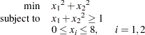Use the following SAS code to solve the problem:

proc optmodel;
   var x {1..2} <= 8 >= 0   /* variable bounds */
      init 0;   /* starting point */
   
   minimize obj = x[1]^2 + x[2]^2;
   
   con cons: 
      x[1] + x[2]^2 >= 1;
   
   solve with sqp / printfreq = 5;
   print x;
quit;

When $\text{[math]}$ = (0, 0) is chosen as the starting point, the SQP solver converges to (1, 0), as displayed in Output 15.2.1. It can be easily verified that (1, 0) is a stationary point and not an optimal solution.

Output 15.2.1 Stationary Point

The OPTMODEL Procedure

Problem Summary
Objective Sense	Minimization
Objective Function	obj
Objective Type	Quadratic

Number of Variables	2
Bounded Above	0
Bounded Below	0
Bounded Below and Above	2
Free	0
Fixed	0

Number of Constraints	1
Linear LE (<=)	0
Linear EQ (=)	0
Linear GE (>=)	0
Linear Range	0
Nonlinear LE (<=)	0
Nonlinear EQ (=)	0
Nonlinear GE (>=)	1
Nonlinear Range	0

Solution Summary
Solver	SQP
Objective Function	obj
Solution Status	Optimal
Objective Value	0.9999999902
Iterations	16

Infeasibility	4.9179166E-9
Optimality Error	1.6715703E-6
Complementarity	4.9179166E-9

[1]	x
1	1
2	0

To resolve this issue, you can use the HESCHECK option in the SOLVE statement as follows:

   proc optmodel;
   ...
      solve with sqp / printfreq = 1 hescheck;
   ...
   quit;

For the same starting point $\text{[math]}$ = (0, 0), the SQP solver now converges to the optimal solution, $\text{[math]}$ , as displayed in Output 15.2.2.

proc optmodel;
   var x {1..2} <= 8 >= 0   /* variable bounds */
      init 0;   /* starting point */
   
   minimize obj = x[1]^2 + x[2]^2;
   
   con cons: 
      x[1] + x[2]^2 >= 1;
   
   solve with sqp / printfreq = 5 hescheck;
   print x;
quit;

Output 15.2.2 Optimal Solution Using the HESCHECK Option

The OPTMODEL Procedure

Problem Summary
Objective Sense	Minimization
Objective Function	obj
Objective Type	Quadratic

Number of Variables	2
Bounded Above	0
Bounded Below	0
Bounded Below and Above	2
Free	0
Fixed	0

Number of Constraints	1
Linear LE (<=)	0
Linear EQ (=)	0
Linear GE (>=)	0
Linear Range	0
Nonlinear LE (<=)	0
Nonlinear EQ (=)	0
Nonlinear GE (>=)	1
Nonlinear Range	0

Solution Summary
Solver	SQP
Objective Function	obj
Solution Status	Optimal
Objective Value	0.7499999978
Iterations	38

Infeasibility	2.2304958E-9
Optimality Error	2.3153477E-6
Complementarity	2.2304958E-9

[1]	x
1	0.5000
2	0.7071

Top of Page