The Sequential Quadratic Programming Solver: Solving a Highly Nonlinear Problem :: SAS/OR(R) 9.22 User's Guide: Mathematical Programming

The Sequential Quadratic Programming Solver

Example 15.1 Solving a Highly Nonlinear Problem

Consider the following example of minimizing a highly nonlinear problem:

$\text{[math]}$

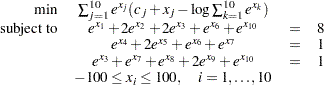In this instance, the constants $\text{[math]}$ are $\text{[math]}$ . Assume the starting point $\text{[math]}$ . You can use the following SAS code to solve the problem:

proc optmodel;
   var x {1..10} >= -100 <= 100   /* variable bounds */
      init -2.3;   /* starting point */

   number c {1..10} = [-6.089 -17.164 -34.054 -5.914 -24.721 
      -14.986 -24.100 -10.708 -26.662 -22.179];
   
   number a{1..3,1..10}=[1 2 2 0 0 1 0 0 0 1
                         0 0 0 1 2 1 1 0 0 0
                         0 0 1 0 0 0 1 1 2 1];
   
   number b{1..3}=[8 1 1];
   
   minimize obj = 
      sum{j in 1..10}exp(x[j])*(c[j]+x[j]
         -log(sum {k in 1..10}exp(x[k])));
   
   con cons{i in 1..3}: 
      sum{j in 1..10}a[i,j]*exp(x[j])=b[i];
   
   solve with sqp / printfreq = 0;
quit;

The output is displayed in Output 15.1.1.

Output 15.1.1 OPTMODEL Output

The OPTMODEL Procedure

Problem Summary
Objective Sense	Minimization
Objective Function	obj
Objective Type	Nonlinear

Number of Variables	10
Bounded Above	0
Bounded Below	0
Bounded Below and Above	10
Free	0
Fixed	0

Number of Constraints	3
Linear LE (<=)	0
Linear EQ (=)	0
Linear GE (>=)	0
Linear Range	0
Nonlinear LE (<=)	0
Nonlinear EQ (=)	3
Nonlinear GE (>=)	0
Nonlinear Range	0

Solution Summary
Solver	SQP
Objective Function	obj
Solution Status	Optimal
Objective Value	-102.0863279
Iterations	80

Infeasibility	4.7356948E-7
Optimality Error	3.3847789E-6
Complementarity	0

Top of Page