| The NLP Procedure |
Example 6.8 Chemical Equilibrium
The following example is used in many test libraries for nonlinear programming and was taken originally from Bracken and McCormick (1968).
The problem is to determine the composition of a mixture of various chemicals satisfying its chemical equilibrium state. The second law of thermodynamics implies that a mixture of chemicals satisfies its chemical equilibrium state (at a constant temperature and pressure) when the free energy of the mixture is reduced to a minimum. Therefore the composition of the chemicals satisfying its chemical equilibrium state can be found by minimizing the function of the free energy of the mixture.
Notation:
|
number of chemical elements in the mixture |
|
number of compounds in the mixture |
|
number of moles for compound |
|
total number of moles in the mixture |
|
number of atoms of element |
|
atomic weight of element |


 in a molecule of compound
Constraints for the Mixture:
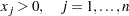
The number of moles must be positive:
There are
 mass balance relationships,
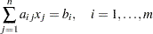
Objective Function: Total Free Energy of Mixture
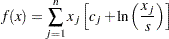 |
with
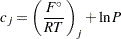 |
where  is the model standard free energy function for the
  th compound (found in tables) and
  is the total pressure in atmospheres.
Minimization Problem:
Determine the parameters  that minimize the objective function
  subject to the nonnegativity and linear balance constraints.
Numeric Example:
Determine the equilibrium composition of compound  at temperature
  and pressure
  .
.
|
||||||
|
|
|
||||
|
Compound |
|
|
|
|
|
1 |
|
-10.021 |
-6.089 |
1 |
||
2 |
|
-21.096 |
-17.164 |
2 |
||
3 |
|
-37.986 |
-34.054 |
2 |
1 |
|
4 |
|
-9.846 |
-5.914 |
1 |
||
5 |
|
-28.653 |
-24.721 |
2 |
||
6 |
|
-18.918 |
-14.986 |
1 |
1 |
|
7 |
|
-28.032 |
-24.100 |
1 |
1 |
|
8 |
|
-14.640 |
-10.708 |
1 |
||
9 |
|
-30.594 |
-26.662 |
2 |
||
10 |
|
-26.111 |
-22.179 |
1 |
1 |
|


Example Specification:
proc nlp tech=tr pall;
      array c[10] -6.089 -17.164 -34.054  -5.914 -24.721
              -14.986 -24.100 -10.708 -26.662 -22.179;
   array x[10] x1-x10;
   min y;
   parms x1-x10 = .1;
   bounds 1.e-6 <= x1-x10;
   lincon 2. = x1 + 2. * x2 + 2. * x3 + x6 + x10,
          1. = x4 + 2. * x5 + x6 + x7,
          1. = x3 + x7  + x8 + 2. * x9 + x10;
   s = x1 + x2 + x3 + x4 + x5 + x6 + x7 + x8 + x9 + x10;
   y = 0.;
   do j = 1 to 10;
      y = y + x[j] * (c[j] + log(x[j] / s));
   end;
run;
Displayed Output:
The iteration history given in Output 6.8.1 does not show any problems.
| Iteration | Restarts | Function Calls |
Active Constraints |
Objective Function |
Objective Function Change |
Max Abs Gradient Element |
Lambda | Trust Region Radius |
||
|---|---|---|---|---|---|---|---|---|---|---|
| 1 | 0 | 2 | 3 | ' | -47.33412 | 2.2790 | 6.0765 | 2.456 | 1.000 | |
| 2 | 0 | 3 | 3 | ' | -47.70043 | 0.3663 | 8.5592 | 0.908 | 0.418 | |
| 3 | 0 | 4 | 3 | -47.73074 | 0.0303 | 6.4942 | 0 | 0.359 | ||
| 4 | 0 | 5 | 3 | -47.73275 | 0.00201 | 4.7606 | 0 | 0.118 | ||
| 5 | 0 | 6 | 3 | -47.73554 | 0.00279 | 3.2125 | 0 | 0.0168 | ||
| 6 | 0 | 7 | 3 | -47.74223 | 0.00669 | 1.9552 | 110.6 | 0.00271 | ||
| 7 | 0 | 8 | 3 | -47.75048 | 0.00825 | 1.1157 | 102.9 | 0.00563 | ||
| 8 | 0 | 9 | 3 | -47.75876 | 0.00828 | 0.4165 | 3.787 | 0.0116 | ||
| 9 | 0 | 10 | 3 | -47.76101 | 0.00224 | 0.0716 | 0 | 0.0121 | ||
| 10 | 0 | 11 | 3 | -47.76109 | 0.000083 | 0.00238 | 0 | 0.0111 | ||
| 11 | 0 | 12 | 3 | -47.76109 | 9.609E-8 | 2.733E-6 | 0 | 0.00248 |
Output 6.8.2 lists the optimal parameters with the gradient.
| Optimization Results | |||
|---|---|---|---|
| Parameter Estimates | |||
| N | Parameter | Estimate | Gradient Objective Function |
| 1 | x1 | 0.040668 | -9.785055 |
| 2 | x2 | 0.147730 | -19.570110 |
| 3 | x3 | 0.783153 | -34.792170 |
| 4 | x4 | 0.001414 | -12.968921 |
| 5 | x5 | 0.485247 | -25.937841 |
| 6 | x6 | 0.000693 | -22.753976 |
| 7 | x7 | 0.027399 | -28.190984 |
| 8 | x8 | 0.017947 | -15.222060 |
| 9 | x9 | 0.037314 | -30.444120 |
| 10 | x10 | 0.096871 | -25.007115 |
The three equality constraints are satisfied at the solution, as shown in Output 6.8.3.
| Linear Constraints Evaluated at Solution | ||||||||||||||||||||||||
|---|---|---|---|---|---|---|---|---|---|---|---|---|---|---|---|---|---|---|---|---|---|---|---|---|
| 1 | ACT | -3.608E-16 | = | 2.0000 | - | 1.0000 | * | x1 | - | 2.0000 | * | x2 | - | 2.0000 | * | x3 | - | 1.0000 | * | x6 | - | 1.0000 | * | x10 |
| 2 | ACT | 2.2204E-16 | = | 1.0000 | - | 1.0000 | * | x4 | - | 2.0000 | * | x5 | - | 1.0000 | * | x6 | - | 1.0000 | * | x7 | ||||
| 3 | ACT | -1.943E-16 | = | 1.0000 | - | 1.0000 | * | x3 | - | 1.0000 | * | x7 | - | 1.0000 | * | x8 | - | 2.0000 | * | x9 | - | 1.0000 | * | x10 |
The Lagrange multipliers are given in Output 6.8.4.
| First Order Lagrange Multipliers | ||
|---|---|---|
| Active Constraint | Lagrange Multiplier |
|
| Linear EC | [1] | 9.785055 |
| Linear EC | [2] | 12.968921 |
| Linear EC | [3] | 15.222060 |
The elements of the projected gradient must be small to satisfy a necessary first-order optimality condition. The projected gradient is given in Output 6.8.5.
| Projected Gradient | |
|---|---|
| Free Dimension |
Projected Gradient |
| 1 | 4.5770108E-9 |
| 2 | 6.868355E-10 |
| 3 | -7.283013E-9 |
| 4 | -0.000001864 |
| 5 | -0.000001434 |
| 6 | -0.000001361 |
| 7 | -0.000000294 |
The projected Hessian matrix shown in Output 6.8.6 is positive definite, satisfying the second-order optimality condition.
| Projected Hessian Matrix | |||||||
|---|---|---|---|---|---|---|---|
| X1 | X2 | X3 | X4 | X5 | X6 | X7 | |
| X1 | 20.903196985 | -0.122067474 | 2.6480263467 | 3.3439156526 | -1.373829641 | -1.491808185 | 1.1462413516 |
| X2 | -0.122067474 | 565.97299938 | 106.54631863 | -83.7084843 | -37.43971036 | -36.20703737 | -16.635529 |
| X3 | 2.6480263467 | 106.54631863 | 1052.3567179 | -115.230587 | 182.89278895 | 175.97949593 | -57.04158208 |
| X4 | 3.3439156526 | -83.7084843 | -115.230587 | 37.529977667 | -4.621642366 | -4.574152161 | 10.306551561 |
| X5 | -1.373829641 | -37.43971036 | 182.89278895 | -4.621642366 | 79.326057844 | 22.960487404 | -12.69831637 |
| X6 | -1.491808185 | -36.20703737 | 175.97949593 | -4.574152161 | 22.960487404 | 66.669897023 | -8.121228758 |
| X7 | 1.1462413516 | -16.635529 | -57.04158208 | 10.306551561 | -12.69831637 | -8.121228758 | 14.690478023 |
The following PROC NLP call uses a specified analytical gradient and the Hessian matrix is computed by finite-difference approximations based on the analytic gradient:
proc nlp tech=tr fdhessian all;
   array c[10] -6.089 -17.164 -34.054  -5.914 -24.721
              -14.986 -24.100 -10.708 -26.662 -22.179;
   array x[10] x1-x10;
   array g[10] g1-g10;
   min y;
   parms x1-x10 = .1;
   bounds 1.e-6 <= x1-x10;
   lincon 2. = x1 + 2. * x2 + 2. * x3 + x6 + x10,
          1. = x4 + 2. * x5 + x6 + x7,
          1. = x3 + x7  + x8 + 2. * x9 + x10;
   s = x1 + x2 + x3 + x4 + x5 + x6 + x7 + x8 + x9 + x10;
   y = 0.;
   do j = 1 to 10;
      y = y + x[j] * (c[j] + log(x[j] / s));
      g[j] = c[j] + log(x[j] / s);
   end;
run;
The results are almost identical to those of the previous run.
Copyright © SAS Institute, Inc. All Rights Reserved.