| The NLP Procedure |
Example 6.6 Maximum Likelihood Weibull Estimation
Two-Parameter Weibull Estimation
The following data are taken from Lawless (1982, p. 193) and represent the number of days it took rats painted with a carcinogen to develop carcinoma. The last two observations are censored data from a group of 19 rats:
data pike;
   input days cens @@;
   datalines;
143  0  164  0  188  0  188  0
190  0  192  0  206  0  209  0
213  0  216  0  220  0  227  0
230  0  234  0  246  0  265  0
304  0  216  1  244  1
;
Suppose that you want to show how to compute the maximum likelihood estimates of the scale parameter  (
( in Lawless), the shape parameter
  (
( in Lawless), and the location parameter
  (
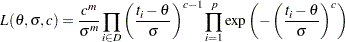
( in Lawless). The observed likelihood function of the three-parameter Weibull transformation (Lawless 1982, p. 191) is
 |
and the log likelihood is
 |
The log likelihood function can be evaluated only for  ,
,  , and
, and  . In the estimation process, you must enforce these conditions using lower and upper boundary constraints. The three-parameter Weibull estimation can be numerically difficult, and it usually pays off to provide good initial estimates. Therefore, you first estimate and of the two-parameter Weibull distribution for constant
  . You then use the optimal parameters
  and
and  as starting values for the three-parameter Weibull estimation.
Although the use of an INEST= data set is not really necessary for this simple example, it illustrates how it is used to specify starting values and lower boundary constraints:
data par1(type=est);
   keep _type_ sig c theta;
   _type_='parms'; sig = .5;
      c = .5; theta = 0; output;
   _type_='lb'; sig = 1.0e-6;
      c = 1.0e-6; theta = .;  output;
run;
The following PROC NLP call specifies the maximization of the log likelihood function for the two-parameter Weibull estimation for constant :
proc nlp data=pike tech=tr inest=par1 outest=opar1
     outmodel=model cov=2 vardef=n pcov phes;
           max logf;
   parms sig c;
   profile sig c / alpha = .9 to .1 by -.1 .09 to .01 by -.01;

   x_th = days - theta;
   s    = - (x_th / sig)**c;
   if cens=0 then s + log(c) - c*log(sig) + (c-1)*log(x_th);
   logf = s;
run;
After a few iterations you obtain the solution given in Output 6.6.1.
| Optimization Results | ||||||
|---|---|---|---|---|---|---|
| Parameter Estimates | ||||||
| N | Parameter | Estimate | Approx Std Err |
t Value | Approx Pr > |t| |
Gradient Objective Function |
| 1 | sig | 234.318611 | 9.645908 | 24.292021 | 9.050475E-16 | 1.3372183E-9 |
| 2 | c | 6.083147 | 1.068229 | 5.694611 | 0.000017269 | -7.859277E-9 |
Since the gradient has only small elements and the Hessian (shown in Output 6.6.2) is negative definite (has only negative eigenvalues), the solution defines an isolated maximum point.

| Hessian Matrix | ||
|---|---|---|
| sig | c | |
| sig | -0.011457556 | 0.0257527577 |
| c | 0.0257527577 | -0.934221388 |
The square roots of the diagonal elements of the approximate covariance matrix of parameter estimates are the approximate standard errors (ASE’s). The covariance matrix is given in Output 6.6.3.
| Covariance Matrix 2: H = (NOBS/d) inv(G) |
||
|---|---|---|
| sig | c | |
| sig | 93.043549863 | 2.5648395794 |
| c | 2.5648395794 | 1.141112488 |
The confidence limits in Output 6.6.4 correspond to the values in the PROFILE statement.
| Wald and PL Confidence Limits | |||||||
|---|---|---|---|---|---|---|---|
| N | Parameter | Estimate | Alpha | Profile Likelihood Confidence Limits |
Wald Confidence Limits | ||
| 1 | sig | 234.318611 | 0.900000 | 233.111324 | 235.532695 | 233.106494 | 235.530729 |
| 1 | sig | . | 0.800000 | 231.886549 | 236.772876 | 231.874849 | 236.762374 |
| 1 | sig | . | 0.700000 | 230.623280 | 238.063824 | 230.601846 | 238.035377 |
| 1 | sig | . | 0.600000 | 229.292797 | 239.436639 | 229.260292 | 239.376931 |
| 1 | sig | . | 0.500000 | 227.855829 | 240.935290 | 227.812545 | 240.824678 |
| 1 | sig | . | 0.400000 | 226.251597 | 242.629201 | 226.200410 | 242.436813 |
| 1 | sig | . | 0.300000 | 224.372260 | 244.643392 | 224.321270 | 244.315953 |
| 1 | sig | . | 0.200000 | 221.984557 | 247.278423 | 221.956882 | 246.680341 |
| 1 | sig | . | 0.100000 | 218.390824 | 251.394102 | 218.452504 | 250.184719 |
| 1 | sig | . | 0.090000 | 217.884162 | 251.987489 | 217.964960 | 250.672263 |
| 1 | sig | . | 0.080000 | 217.326988 | 252.645278 | 217.431654 | 251.205569 |
| 1 | sig | . | 0.070000 | 216.708814 | 253.383546 | 216.841087 | 251.796136 |
| 1 | sig | . | 0.060000 | 216.008815 | 254.228034 | 216.176649 | 252.460574 |
| 1 | sig | . | 0.050000 | 215.199301 | 255.215496 | 215.412978 | 253.224245 |
| 1 | sig | . | 0.040000 | 214.230116 | 256.411041 | 214.508337 | 254.128885 |
| 1 | sig | . | 0.030000 | 213.020874 | 257.935686 | 213.386118 | 255.251105 |
| 1 | sig | . | 0.020000 | 211.369067 | 260.066128 | 211.878873 | 256.758350 |
| 1 | sig | . | 0.010000 | 208.671091 | 263.687174 | 209.472398 | 259.164825 |
| 2 | c | 6.083147 | 0.900000 | 5.950029 | 6.217752 | 5.948912 | 6.217382 |
| 2 | c | . | 0.800000 | 5.815559 | 6.355576 | 5.812514 | 6.353780 |
| 2 | c | . | 0.700000 | 5.677909 | 6.499187 | 5.671537 | 6.494757 |
| 2 | c | . | 0.600000 | 5.534275 | 6.651789 | 5.522967 | 6.643327 |
| 2 | c | . | 0.500000 | 5.380952 | 6.817880 | 5.362638 | 6.803656 |
| 2 | c | . | 0.400000 | 5.212344 | 7.004485 | 5.184103 | 6.982191 |
| 2 | c | . | 0.300000 | 5.018784 | 7.225733 | 4.975999 | 7.190295 |
| 2 | c | . | 0.200000 | 4.776379 | 7.506166 | 4.714157 | 7.452137 |
| 2 | c | . | 0.100000 | 4.431310 | 7.931669 | 4.326067 | 7.840227 |
| 2 | c | . | 0.090000 | 4.382687 | 7.991457 | 4.272075 | 7.894220 |
| 2 | c | . | 0.080000 | 4.327815 | 8.056628 | 4.213014 | 7.953280 |
| 2 | c | . | 0.070000 | 4.270773 | 8.129238 | 4.147612 | 8.018682 |
| 2 | c | . | 0.060000 | 4.207130 | 8.211221 | 4.074029 | 8.092265 |
| 2 | c | . | 0.050000 | 4.134675 | 8.306218 | 3.989457 | 8.176837 |
| 2 | c | . | 0.040000 | 4.049531 | 8.418782 | 3.889274 | 8.277021 |
| 2 | c | . | 0.030000 | 3.945037 | 8.559677 | 3.764994 | 8.401300 |
| 2 | c | . | 0.020000 | 3.805759 | 8.749130 | 3.598076 | 8.568219 |
| 2 | c | . | 0.010000 | 3.588814 | 9.056751 | 3.331572 | 8.834722 |
Three-Parameter Weibull Estimation
You now prepare for the three-parameter Weibull estimation by using PROC UNIVARIATE to obtain the smallest data value for the upper boundary constraint for . For this small problem, you can do this much more simply by just using a value slightly smaller than the minimum data value 143.
/* Calculate upper bound for theta parameter */
proc univariate data=pike noprint;
   var days;
   output out=stats n=nobs min=minx range=range;
run;
data stats;
   set stats;
   keep _type_ theta;

   /* 1. write parms observation */
   theta = minx - .1 * range;
   if theta < 0 then theta = 0;
   _type_ = 'parms';
   output;

   /* 2. write ub observation */
   theta = minx * (1 - 1e-4);
   _type_ = 'ub';
   output;
run;
The data set PAR2 specifies the starting values and the lower and upper bounds for the three-parameter Weibull problem:
proc sort data=opar1;
   by _type_;
run;
data par2(type=est);
   merge opar1(drop=theta) stats;
   by _type_;
   keep _type_ sig c theta;
   if _type_ in ('parms' 'lowerbd' 'ub');
run;
The following PROC NLP call uses the MODEL= input data set containing the log likelihood function that was saved during the two-parameter Weibull estimation:
proc nlp data=pike tech=tr inest=par2 outest=opar2
      model=model cov=2 vardef=n pcov phes;
   max logf;
   parms sig c theta;
   profile sig c theta / alpha = .5 .1 .05 .01;
run;
After a few iterations, you obtain the solution given in Output 6.6.5.
| Optimization Results | ||||||
|---|---|---|---|---|---|---|
| Parameter Estimates | ||||||
| N | Parameter | Estimate | Approx Std Err |
t Value | Approx Pr > |t| |
Gradient Objective Function |
| 1 | sig | 108.382690 | 32.573321 | 3.327345 | 0.003540 | -3.132469E-9 |
| 2 | c | 2.711476 | 1.058757 | 2.560998 | 0.019108 | -0.000000487 |
| 3 | theta | 122.025982 | 28.692364 | 4.252908 | 0.000430 | -6.760135E-8 |
From inspecting the first- and second-order derivatives at the optimal solution, you can verify that you have obtained an isolated maximum point. The Hessian matrix is shown in Output 6.6.6.
| Hessian Matrix | |||
|---|---|---|---|
| sig | c | theta | |
| sig | -0.010639963 | 0.045388887 | -0.01003374 |
| c | 0.045388887 | -4.07872453 | -0.083028097 |
| theta | -0.01003374 | -0.083028097 | -0.014752243 |
The square roots of the diagonal elements of the approximate covariance matrix of parameter estimates are the approximate standard errors. The covariance matrix is given in Output 6.6.7.
| Covariance Matrix 2: H = (NOBS/d) inv(G) | |||
|---|---|---|---|
| sig | c | theta | |
| sig | 1060.9795634 | 29.924959631 | -890.0493649 |
| c | 29.924959631 | 1.1209334438 | -26.66229938 |
| theta | -890.0493649 | -26.66229938 | 823.21458961 |
The difference between the Wald and profile CLs for parameter PHI2 are remarkable, especially for the upper 95% and 99% limits, as shown in Output 6.6.8.
| Wald and PL Confidence Limits | |||||||
|---|---|---|---|---|---|---|---|
| N | Parameter | Estimate | Alpha | Profile Likelihood Confidence Limits |
Wald Confidence Limits | ||
| 1 | sig | 108.382732 | 0.500000 | 91.811562 | 141.564605 | 86.412310 | 130.353154 |
| 1 | sig | . | 0.100000 | 76.502373 | . | 54.804263 | 161.961200 |
| 1 | sig | . | 0.050000 | 72.215845 | . | 44.540049 | 172.225415 |
| 1 | sig | . | 0.010000 | 64.262384 | . | 24.479224 | 192.286240 |
| 2 | c | 2.711477 | 0.500000 | 2.139297 | 3.704052 | 1.997355 | 3.425599 |
| 2 | c | . | 0.100000 | 1.574162 | 9.250072 | 0.969973 | 4.452981 |
| 2 | c | . | 0.050000 | 1.424853 | 19.516170 | 0.636347 | 4.786607 |
| 2 | c | . | 0.010000 | 1.163096 | 19.540685 | -0.015706 | 5.438660 |
| 3 | theta | 122.025942 | 0.500000 | 91.027144 | 135.095454 | 102.673186 | 141.378698 |
| 3 | theta | . | 0.100000 | . | 141.833769 | 74.831079 | 142.985700 |
| 3 | theta | . | 0.050000 | . | 142.512603 | 65.789795 | 142.985700 |
| 3 | theta | . | 0.010000 | . | 142.967407 | 48.119116 | 142.985700 |
Copyright © SAS Institute, Inc. All Rights Reserved.