The OPTQP Procedure

Getting Started: OPTQP Procedure

Consider a small illustrative example. Suppose you want to minimize a two-variable quadratic function on the nonnegative quadrant, subject to two constraints:

$\min & 2x_1 & + & 3x_2 & + & x_1^2 & + & 10x_2^2 & + & 2.5 x_1 x_2 \ {subject ... ...& 100 & & & & \ & x_1 & & & \ge & 0 & & & & \ & & & x_2 & \ge & 0 & & & &$

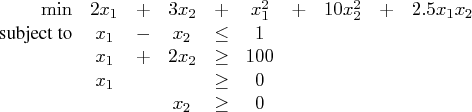
The linear objective function coefficients, vector of right-hand sides, and lower and upper bounds are identified immediately as

$\mathbf{c} = [2 \ 3 ], \mathbf{b} = [1 \ 100 ], \mathbf{l} = [0 \ 0 ], \mathbf{u} = [+\infty \ +\infty ]$

Let us carefully construct the quadratic matrix $\mathbf{q}$ . Observe that you can use symmetry to separate the main-diagonal and off-diagonal elements:

$\frac{1}2 \mathbf{x}^{\rm t} \mathbf{qx} \equiv \frac{1}2 \sum_{i, j = 1}^n\; ... ...\frac{1}2 \sum_{i = 1}^n\; q_{ii}\, x_i^2 + \sum_{i \gt j}\; x_i\, q_{ij}\, x_j$

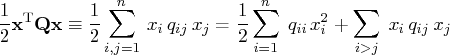
The first expression

$\frac{1}2 \sum_{i = 1}^n\; q_{ii}\, x_i^2$

sums the main-diagonal elements. Thus in this case you have

$q_{11} = 2, q_{22} = 20$

Notice that the main-diagonal values are doubled in order to accommodate the 1/2 factor. Now the second term

$\sum_{i \gt j} x_i\, q_{ij}\, x_j$

sums the off-diagonal elements in the strict lower triangular part of the matrix. The only off-diagonal ( $x_i\, x_j,\; i\not=j$ ) term in the objective function is $2.5\, x_1\, x_2$ , so you have

$q_{21} = 2.5$

Notice that you do not need to specify the upper triangular part of the quadratic matrix.

Finally, the matrix of constraints is as follows:

$\mathbf{a} = [1 & -1 \ 1 & 2 ]$

The QPS-format SAS input data set for the preceding problem can be expressed in the following manner:

 data gsdata;
    input field1 $ field2 $ field3$ field4 field5 $ field6 @;
 datalines;
 NAME   .      EXAMPLE   .             .         .
 ROWS   .      .         .             .         .
 N      OBJ    .         .             .         .
 L      R1     .         .             .         .
 G      R2     .         .             .         .
 COLUMNS .     .         .             .         .
 .      X1     R1         1.0           R2        1.0 
 .      X1     OBJ        2.0           .         .
 .      X2     R1        -1.0           R2        2.0
 .      X2     OBJ        3.0           .         .
 RHS    .      .         .              .         .
 .      RHS    R1        1.0            .         .
 .      RHS    R2        100            .         .
 RANGES .      .         .              .         .
 BOUNDS .      .         .              .         .
 QUADOBJ .     .         .              .         .
 .      X1     X1        2.0            .         .
 .      X1     X2        2.5            .         .
 .      X2     X2        20             .         .
 ENDATA .      .         .              .         .
 ;

For more details about the QPS-format data set, see Chapter 14, "The MPS-Format SAS Data Set."

Alternatively, if you have a QPS-format flat file named gs.qps, then the following call to the SAS macro %MPS2SASD translates that file into a SAS data set, named gsdata:

  
 %mps2sasd(mpsfile =gs.qps, outdata = gsdata);

Note: The SAS macro %MPS2SASD is provided in SAS/OR software. See the section "Converting an MPS/QPS-Format File: %MPS2SASD" for details.

You can use the following call to PROC OPTQP:

    proc optqp data=gsdata 
      primalout = gspout 
      dualout   = gsdout;
    run;

The procedure output is displayed in Figure 17.2.

The OPTQP Procedure

Problem Summary
Problem Name	EXAMPLE
Objective Sense	Minimization
Objective Function	OBJ
RHS	RHS

Number of Variables	2
Bounded Above	0
Bounded Below	2
Bounded Above and Below	0
Free	0
Fixed	0

Number of Constraints	2
LE (<=)	1
EQ (=)	0
GE (>=)	1
Range	0

Constraint Coefficients	4

Hessian Diagonal Elements	2
Hessian Elements Above the Diagonal	1

The OPTQP Procedure

Solution Summary
Objective Function	OBJ
Solution Status	Optimal
Objective Value	15018.000761

Primal Infeasibility	0
Dual Infeasibility	0
Bound Infeasibility	0
Duality Gap	9.9575984E-8
Complementarity	0.0014952645

Iterations	10
Presolve Time	0.00
Solution Time	0.02

Figure 17.2: Procedure Output

The optimal primal solution is displayed in Figure 17.3.

Primal Solution

Obs	Objective Function ID	RHS ID	Variable Name	Variable Type	Linear Objective Coefficient	Lower Bound	Upper Bound	Variable Value	Variable Status
1	OBJ	RHS	X1	N	2	0	1.7977E308	34.0000	O
2	OBJ	RHS	X2	N	3	0	1.7977E308	33.0000	O

Figure 17.3: Optimal Solution

The SAS log shown in Figure 17.4 provides information about the problem, convergence information after each iteration, and the optimal objective value.


NOTE: The problem EXAMPLE has 2 variables (0 free, 0 fixed).
NOTE: The problem has 2 constraints (1 LE, 0 EQ, 1 GE, 0 range).
NOTE: The problem has 4 constraint coefficients.
NOTE: The objective function has 2 Hessian diagonal elements and 1 Hessian
elements above the diagonal.
NOTE: The OPTQP presolver value AUTOMATIC is applied.
NOTE: The OPTQP presolver removed 0 variables and 0 constraints.
NOTE: The OPTQP presolver removed 0 constraint coefficients.
NOTE: The QUADRATIC ITERATIVE solver is called.
Primal Bound Dual
Iter Complement Duality Gap Infeas Infeas Infeas
0 63669937 1.985060 0 0 0
1 12781299 1.952937 0 0 0
2 2189517 1.877587 0 0 0
3 363689 1.669055 0 0 0
4 57278 1.058687 0 0 0
5 5621.204805 0.239307 0 0 0
6 914.397217 0.015841 0 0 0
7 14.822037 0.000796 0 0 0
8 0.605195 0.000039820 0 0 0
9 0.029919 0.000001991 0 0 0
10 0.001495 9.9575984E-8 0 0 0
NOTE: Optimal.
NOTE: Objective = 15018.000761.

Figure 17.4: Iteration Log

See the section "Interior Point Algorithm: Overview" and the section "Iteration Log for the OPTQP Procedure" for more details about convergence information given by the iteration log.

Top of Page