PROC OPTQP: Example 17.1: Linear Least-Squares Problem :: SAS/OR(R) 9.2 User's Guide: Mathematical Programming

The OPTQP Procedure

Example 17.1: Linear Least-Squares Problem

The linear least-squares problem arises in the context of determining a solution to an over-determined set of linear equations. In practice, these could arise in data fitting and estimation problems. An 1 system of linear equations can be defined as

$\mathbf{ax} = \mathbf{b}$

where $\mathbf{a} \in \mathbb{r}^{m x n}$ , $\mathbf{x}\in \mathbb{r}^n$ , $\mathbf{b} \in \mathbb{r}^m$ , and $m \gt n$ . Since this system usually does not have a solution, we need to be satisfied with some sort of approximate solution. The most widely used approximation is the least-squares solution, which minimizes $\vert \mathbf{ax} - \mathbf{b}\vert _2^2$ .

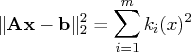
This problem is called a least-squares problem for the following reason. Let $\mathbf{a}$ , $\mathbf{x}$ , and $\mathbf{b}$ be defined as previously. Let be the th component of the vector $\mathbf{ax} - \mathbf{b}$ :

$k_i(x) = a_{i1}x_1 + a_{i2}x_2 + ... + a_{in}x_n - b_i,\; i = 1,2, ... , m$

By definition of the Euclidean norm, the objective function can be expressed as follows:

$\vert \mathbf{ax} - \mathbf{b}\vert _2^2 = \sum \limits_{i = 1}^m k_i(x)^2$

Therefore, the function we minimize is the sum of squares of

terms

; hence the term least-squares. The following example is an illustration of the linear least-squares problem; i.e., each of the terms

is a linear function of

.Consider the following least-squares problem defined by

$\mathbf{a} = [4 & 0 \ -1 & 1 \ 3 & 2 ], \mathbf{b} = [1 \ 0 \ 1 ]$

This translates to the following set of linear equations:

The corresponding least-squares problem is

${minimize} (4x_1 -1)^2 + (-x_1 + x_2)^2 + (3x_1 + 2x_2 -1)^2$

The preceding objective function can be expanded to

${minimize} 26x_1^2 + 5x_2^2 + 10 x_1x_2 - 14 x_1 -4x_2 + 2$

In addition, we impose the following constraint so that the equation

is satisfied within a tolerance of 0.1:

$0.9 \leq 3x_1 + 2x_2 \leq 1.1$

You can create the QPS-format input data set by using the following SAS code:

 data lsdata;
    input field1 $ field2 $ field3$ field4 field5 $ field6 @;
 datalines;
 NAME   .      LEASTSQ     .            .         .
 ROWS   .      .           .            .         .
 N      OBJ    .           .            .         .
 G      EQ3    .           .            .         .
 COLUMNS .     .           .            .         .
 .      X1     OBJ       -14            EQ3       3
 .      X2     OBJ        -4            EQ3       2
 RHS    .      .           .            .         .
 .      RHS    OBJ        -2            EQ3     0.9
 RANGES .      .           .            .         .
 .      RNG    EQ3       0.2            .         .
 BOUNDS .      .           .            .         .
 FR    BND1    X1          .            .         .
 FR    BND1    X2          .            .         .
 QUADOBJ .     .           .            .         .
 .      X1     X1         52            .         .
 .      X1     X2         10            .         .
 .      X2     X2         10            .         .
 ENDATA .      .           .            .         .
 ;

The decision variables and are free, so they have bound type FR in the BOUNDS section of the QPS-format data set.

You can use the following SAS code to solve the least-squares problem:

    proc optqp data=lsdata 
      primalout = lspout; 
    run;

The optimal solution is displayed in Output 17.1.1.

Output 17.1.1: Solution to the Least-Squares Problem

Primal Solution

Obs	Objective Function ID	RHS ID	Variable Name	Variable Type	Linear Objective Coefficient	Lower Bound	Upper Bound	Variable Value	Variable Status
1	OBJ	RHS	X1	F	-14	-1.7977E308	1.7977E308	0.23809	O
2	OBJ	RHS	X2	F	-4	-1.7977E308	1.7977E308	0.16190	O

The iteration log is shown in Output 17.1.2.

Output 17.1.2: Iteration Log


NOTE: The problem LEASTSQ has 2 variables (2 free, 0 fixed).
NOTE: The problem has 1 constraints (0 LE, 0 EQ, 0 GE, 1 range).
NOTE: The problem has 2 constraint coefficients.
NOTE: The objective function has 2 Hessian diagonal elements and 1 Hessian
elements above the diagonal.
NOTE: The OPTQP presolver value AUTOMATIC is applied.
NOTE: The OPTQP presolver removed 0 variables and 0 constraints.
NOTE: The OPTQP presolver removed 0 constraint coefficients.
NOTE: The QUADRATIC ITERATIVE solver is called.
Primal Bound Dual
Iter Complement Duality Gap Infeas Infeas Infeas
0 10001805 2.001029 1052.607895 416.588001 0
1 501893 2.094827 52.630395 20.750266 0
2 26887 34.114879 2.631520 0.958349 0
3 2997.321110 600.993085 0.131576 0 0
4 734.867262 111.975745 0.006579 0 0
5 26.413788 5.701869 0.000329 0 0
6 0.877292 0.287945 0.000016608 0 0
7 0.051222 0.017041 0.000000983 0 0
8 0.007624 0.001934 0.000000103 0 0
9 0.001232 0.000171 5.7776383E-9 0 0
10 0.000047950 0.000008773 2.898554E-10 0 0
11 0.000001381 0.000000438 1.449273E-11 0 0
NOTE: Optimal.
NOTE: Objective = 0.0095238096.

Top of Page