The NLP Procedure

Example 4.9: Minimize Total Delay in a Network

The following example is taken from the user's guide of GINO (Liebman et al. 1986). A simple network of five roads (arcs) can be illustrated by the path diagram:

Figure 4.11: Simple Road Network

The five roads connect four intersections illustrated by numbered nodes. Each minute vehicles enter and leave the network. Arc refers to the road from intersection to intersection , and the parameter refers to the flow from to . The law that traffic flowing into each intersection must also flow out is described by the linear equality constraint

In general, roads also have an upper capacity, which is the number of vehicles which can be handled per minute. The upper limits can be enforced by boundary constraints

Finding the maximum flow through a network is equivalent to solving a simple linear optimization problem, and for large problems, PROC LP or PROC NETFLOW can be used. The objective function is

and the constraints are

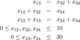
The three linear equality constraints are linearly dependent. One of them is deleted automatically by the PROC NLP subroutines. Even though the default technique is used for this small example, any optimization subroutine can be used.

  
    proc nlp all initial=.5; 
       max y; 
       parms x12 x13 x32 x24 x34; 
       bounds x12 <= 10, 
              x13 <= 30, 
              x32 <= 10, 
              x24 <= 30, 
              x34 <= 10; 
       /* what flows into an intersection must flow out */ 
       lincon x13 = x32 + x34, 
              x12 + x32 = x24, 
              x24 + x34 = x12 + x13; 
       y = x24 + x34 + 0*x12 + 0*x13 + 0*x32; 
    run;
 

The iteration history is given in Output 4.9.1, and the optimal solution is given in Output 4.9.2.

Output 4.9.1: Iteration History

Newton-Raphson Ridge Optimization Without Parameter Scaling Iteration   Restarts Function Calls Active Constraints   Objective Function Objective Function Change Max Abs Gradient Element Ridge Ratio Between Actual and Predicted Change 1 * 0 2 4   20.25000 19.2500 0.5774 0.0313 0.860 2 * 0 3 5   30.00000 9.7500 0 0.0313 1.683 Optimization Results Iterations 2 Function Calls 4 Hessian Calls 3 Active Constraints 5 Objective Function 30 Max Abs Gradient Element 0 Ridge 0 Actual Over Pred Change 1.6834532374 All parameters are actively constrained. Optimization cannot proceed.

Output 4.9.2: Optimization Results

PROC NLP: Nonlinear Maximization Optimization Results Parameter Estimates N Parameter Estimate Gradient Objective Function Active Bound Constraint 1 x12 10.000000 0 Upper BC 2 x13 20.000000 0   3 x32 10.000000 0 Upper BC 4 x24 20.000000 1.000000   5 x34 10.000000 1.000000 Upper BC Value of Objective Function = 30

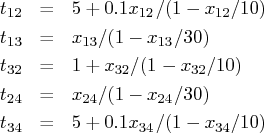
Finding a traffic pattern that minimizes the total delay to move vehicles per minute from node 1 to node 4 introduces nonlinearities that, in turn, demand nonlinear optimization techniques. As traffic volume increases, speed decreases. Let be the travel time on arc and assume that the following formulas describe the travel time as decreasing functions of the amount of traffic:

These formulas use the road capacities (upper bounds), assuming vehicles per minute have to be moved through the network. The objective function is now

and the constraints are

Again, the default algorithm is used:

  
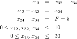
    proc nlp all initial=.5; 
       min y; 
       parms x12 x13 x32 x24 x34; 
       bounds x12 x13 x32 x24 x34 >= 0; 
       lincon x13 = x32 + x34,  /* flow in = flow out */ 
              x12 + x32 = x24, 
              x24 + x34 = 5;    /* = f = desired flow */ 
       t12 = 5 + .1 * x12 / (1 - x12 / 10); 
       t13 = x13 / (1 - x13 / 30); 
       t32 = 1 + x32 / (1 - x32 / 10); 
       t24 = x24 / (1 - x24 / 30); 
       t34 = 5 + .1 * x34 / (1 - x34 / 10); 
       y = t12*x12 + t13*x13 + t32*x32 + t24*x24 + t34*x34; 
    run;
 

The iteration history is given in Output 4.9.3, and the optimal solution is given in Output 4.9.4.

Output 4.9.3: Iteration History

Newton-Raphson Ridge Optimization Without Parameter Scaling Iteration   Restarts Function Calls Active Constraints   Objective Function Objective Function Change Max Abs Gradient Element Ridge Ratio Between Actual and Predicted Change 1   0 2 4   40.30303 0.3433 4.44E-16 0 0.508 Optimization Results Iterations 1 Function Calls 3 Hessian Calls 2 Active Constraints 4 Objective Function 40.303030303 Max Abs Gradient Element 4.440892E-16 Ridge 0 Actual Over Pred Change 0.5083585587 ABSGCONV convergence criterion satisfied.

Output 4.9.4: Optimization Results

PROC NLP: Nonlinear Minimization Optimization Results Parameter Estimates N Parameter Estimate Gradient Objective Function Active Bound Constraint 1 x12 2.500000 5.777778   2 x13 2.500000 5.702479   3 x32 1.114018E-17 1.000000 Lower BC 4 x24 2.500000 5.702479   5 x34 2.500000 5.777778   Value of Objective Function = 40.303030303

The active constraints and corresponding Lagrange multiplier estimates (costs) are given in Output 4.9.5 and Output 4.9.6, respectively.

Output 4.9.5: Linear Constraints at Solution

PROC NLP: Nonlinear Minimization Linear Constraints Evaluated at Solution 1 ACT 4.4409E-16 = 0 + 1.0000 * x13 - 1.0000 * x32 - 1.0000 * x34 2 ACT 4.4409E-16 = 0 + 1.0000 * x12 + 1.0000 * x32 - 1.0000 * x24 3 ACT 0 = -5.0000 + 1.0000 * x24 + 1.0000 * x34

Output 4.9.6: Lagrange Multipliers at Solution

First Order Lagrange Multipliers Active Constraint Lagrange Multiplier Lower BC x32 0.924702 Linear EC [1] 5.702479 Linear EC [2] 5.777778 Linear EC [3] 11.480257

Output 4.9.7 shows that the projected gradient is very small, satisfying the first-order optimality criterion.

Output 4.9.7: Projected Gradient at Solution

Projected Gradient Free Dimension Projected Gradient 1 4.440892E-16

The projected Hessian matrix (shown in Output 4.9.8) is positive definite, satisfying the second-order optimality criterion.

Output 4.9.8: Projected Hessian at Solution

Projected Hessian Matrix   X1 X1 1.535309013