PROC NETFLOW: Network Models: Interior Point Algorithm :: SAS/OR(R) 9.2 User's Guide: Mathematical Programming

The NETFLOW Procedure

Network Models: Interior Point Algorithm

The data required by PROC NETFLOW for a network problem is identical whether the simplex algorithm or the interior point algorithm is used as the optimizer. By default, the simplex algorithm is used for problems with a network component. To use the interior point algorithm, all you need to do is specify the INTPOINT option in the PROC NETFLOW statement. You can optionally specify some options that control the interior point algorithm, of which there are only a few. The interior point algorithm is remarkably robust when reasonable choices are made during the design and implementation, so it does not need to be tuned to the same extent as the simplex algorithm.

When to Use INTPOINT: Network Models: Interior Point Algorithm

PROC NETFLOW uses the primal simplex network algorithm and the primal partitioning algorithm to solve constrained network problems. These algorithms are fast, since they take advantage of algebraic properties of the network component of the problem.

If the network component of the model is large compared to the side constraint component, PROC NETFLOW's optimizer can store what would otherwise be a large matrix as a spanning tree computer data structure. Computations involving the spanning tree data structure can be performed much faster than those using matrices. Only the nonnetwork part of the problem, hopefully quite small, needs to be manipulated by PROC NETFLOW as matrices.

In contrast, LP optimizers must contend with matrices that can be large for large problems. Arithmetic operations on matrices often accumulate rounding errors that cause difficulties for the algorithm. So in addition to the performance improvements, network optimization is generally more numerically stable than LP optimization.

The nodal flow conservation constraints do not need to be specified in the network model. They are implied by the network structure. However, flow conservation constraints do make up the data for the equivalent LP model. If you have an LP that is small after the flow conservation constraints are removed, that problem is a definite candidate for solution by PROC NETFLOW's specialized simplex method.

However, some constrained network problems are solved more quickly by the interior point algorithm than the network optimizer in PROC NETFLOW. Usually, they have a large number of side constraints or nonarc variables. These models are more like LPs than network problems. The network component of the problem is so small that PROC NETFLOW's network simplex method cannot recoup the effort to exploit that component rather than treat the whole problem as an LP. If this is the case, it is worthwhile to get PROC NETFLOW to convert a constrained network problem to the equivalent LP and use its interior point algorithm. This conversion must be done before any optimization has been performed (specify the INTPOINT option in the PROC NETFLOW statement).

Even though some network problems are better solved by converting them to an LP, the input data and the output solution are more conveniently maintained as networks. You retain the advantages of casting problems as networks: ease of problem generation and expansion when more detail is required. The model and optimal solutions are easy to understand, as a network can be drawn.

Getting Started: Network Models: Interior Point Algorithm

To solve network programming problems with side constraints using PROC NETFLOW, you save a representation of the network and the side constraints in three SAS data sets. These data sets are then passed to PROC NETFLOW for solution. There are various forms that a problem's data can take. You can use any one or a combination of several of these forms.

The NODEDATA= data set contains the names of the supply and demand nodes and the supply or demand associated with each. These are the elements in the column vector in problem (NPSC).

The ARCDATA= data set contains information about the variables of the problem. Usually these are arcs, but there can be data related to nonarc variables in the ARCDATA= data set as well. If there are no arcs, this is a linear programming problem.

An arc is identified by the names of its tail node (where it originates) and head node (where it is directed). Each observation can be used to identify an arc in the network and, optionally, the cost per flow unit across the arc, the arc's lower flow bound, capacity, and name. These data are associated with the matrix and the vectors , , and in problem (NPSC).

Note: Although is a node-arc incidence matrix, it is specified in the ARCDATA= data set by arc definitions. Do not explicitly specify these flow conservation constraints as constraints of the problem.

In addition, the ARCDATA= data set can be used to specify information about nonarc variables, including objective function coefficients, lower and upper value bounds, and names. These data are the elements of the vectors , , and in problem (NPSC). Data for an arc or nonarc variable can be given in more than one observation.

Supply and demand data also can be specified in the ARCDATA= data set. In such a case, the NODEDATA= data set may not be needed.

The CONDATA= data set describes the side constraints and their right-hand sides. These data are elements of the matrices and and the vector . Constraint types are also specified in the CONDATA= data set. You can include in this data set upper bound values or capacities, lower flow or value bounds, and costs or objective function coefficients. It is possible to give all information about some or all nonarc variables in the CONDATA= data set.

An arc or nonarc variable is identified in this data set by its name. If you specify an arc's name in the ARCDATA= data set, then this name is used to associate data in the CONDATA= data set with that arc. Each arc also has a default name that is the name of the tail and head node of the arc concatenated together and separated by an underscore character; tail_head, for example.

If you use the dense side constraint input format and want to use the default arc names, these arc names are names of SAS variables in the VAR list of the CONDATA= data set.

If you use the sparse side constraint input format (described later as well) and want to use the default arc names, these arc names are values of the COLUMN list SAS variable of the CONDATA= data set.

When using the interior point algorithm, the execution of PROC NETFLOW has two stages. In the preliminary (zeroth) stage, the data are read from the NODEDATA= data set, the ARCDATA= data set, and the CONDATA= data set. Error checking is performed. The model is converted into an equivalent linear program.

In the next stage, the linear program is preprocessed. This is optional but highly recommended. Preprocessing analyzes the model and tries to determine before optimization whether variables can be "fixed" to their optimal values. Knowing that, the model can be modified and these variables dropped out. It can be determined that some constraints are redundant. Sometimes, preprocessing succeeds in reducing the size of the problem, thereby making the subsequent optimization easier and faster.

The optimal solution to the linear program is then found. The linear program is converted back to the original constrained network problem, and the optimum for this is derived from the optimum of the equivalent linear program. If the problem was preprocessed, the model is now post-processed, where fixed variables are reintroduced. The solution can be saved in the CONOUT= data set. This data set is also named in the PROC NETFLOW, RESET, and SAVE statements.

The interior point algorithm cannot efficiently be warm started, so options such as FUTURE1 and FUTURE2 options are irrelevant.

Introductory Example: Network Models: Interior Point Algorithm

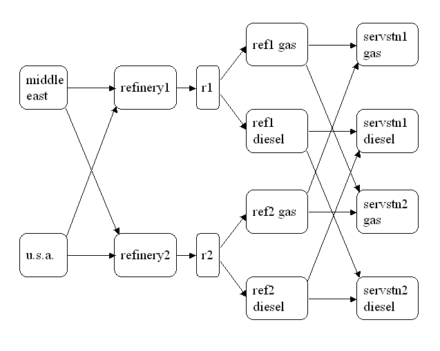
Consider the following transshipment problem for an oil company in the section "Introductory Example". Recall that crude oil is shipped to refineries where it is processed into gasoline and diesel fuel. The gasoline and diesel fuel are then distributed to service stations. At each stage there are shipping, processing, and distribution costs. Also, there are lower flow bounds and capacities. In addition, there are side constraints to model crude mix stipulations, and model the limitations on the amount of Middle Eastern crude that can be processed by each refinery and the conversion proportions of crude to gasoline and diesel fuel. The network diagram is reproduced in Figure 5.16.

Figure 5.16: Oil Industry Example

To solve this problem with PROC NETFLOW, a representation of the model is saved in three SAS data sets that are identical to the data sets supplied to PROC NETFLOW when the simplex algorithm was used.

To find the minimum cost flow through the network that satisfies the supplies, demands, and side constraints, invoke PROC NETFLOW as follows:

  
   proc netflow 
      intpoint              /* <<<--- Interior Point used */ 
      nodedata=noded        /* the supply and demand data */ 
      arcdata=arcd1         /* the arc descriptions       */ 
      condata=cond1         /* the side constraints       */ 
      conout=solution;      /* the solution data set      */ 
      run;

The following messages, which appear on the SAS log, summarize the model as read by PROC NETFLOW and note the progress toward a solution:

  
   NOTE: Number of nodes= 14 . 
   NOTE: Number of supply nodes= 2 . 
   NOTE: Number of demand nodes= 4 . 
   NOTE: Total supply= 180 , total demand= 180 . 
   NOTE: Number of arcs= 18 . 
   NOTE: Number of <= side constraints= 0 . 
   NOTE: Number of == side constraints= 2 . 
   NOTE: Number of >= side constraints= 2 . 
   NOTE: Number of side constraint coefficients= 8 . 
   NOTE: The following messages relate to the equivalent Linear 
         Programming problem solved by the Interior Point 
         algorithm. 
   NOTE: Number of <= constraints= 0 . 
   NOTE: Number of == constraints= 16 . 
   NOTE: Number of >= constraints= 2 . 
   NOTE: Number of constraint coefficients= 44 . 
   NOTE: Number of variables= 18 . 
   NOTE: After preprocessing, number of <= constraints= 0. 
   NOTE: After preprocessing, number of == constraints= 5. 
   NOTE: After preprocessing, number of >= constraints= 2. 
   NOTE: The preprocessor eliminated 11 constraints from the 
         problem. 
   NOTE: The preprocessor eliminated 25 constraint coefficients 
         from the problem. 
   NOTE: After preprocessing, number of variables= 8. 
   NOTE: The preprocessor eliminated 10 variables from the 
         problem. 
   NOTE: 2 columns, 0 rows and 2 coefficients were added to the 
         problem to handle unrestricted variables, variables that 
         are split, and constraint slack or surplus variables. 
   NOTE: There are 13 nonzero elements in A * A transpose. 
   NOTE: Of the 7 rows and columns, 2 are sparse. 
   NOTE: There are 6 nonzero superdiagonal elements in the 
         sparse rows of the factored A * A transpose. This 
         includes fill-in. 
   NOTE: There are 2 operations of the form 
         u[i,j]=u[i,j]-u[q,j]*u[q,i]/u[q,q] to factorize the 
         sparse rows of A * A transpose. 
   NOTE: Bound feasibility attained by iteration 1. 
   NOTE: Dual feasibility attained by iteration 1. 
   NOTE: Constraint feasibility attained by iteration 2. 
   NOTE: The Primal-Dual Predictor-Corrector Interior Point 
         algorithm performed 7 iterations. 
   NOTE: Objective= 50875.01279. 
   NOTE: The data set WORK.SOLUTION has 18 observations and 
         10 variables.

The first set of messages provide statistics on the size of the equivalent linear programming problem. The number of variables may not equal the number of arcs if the problem has nonarc variables. This example has none. To convert a network to an equivalent LP problem, a flow conservation constraint must be created for each node (including an excess or bypass node, if required). This explains why the number of equality side constraints and the number of constraint coefficients change when the interior point algorithm is used.

If the preprocessor was successful in decreasing the problem size, some messages will report how well it did. In this example, the model size was cut in half!

The following set of messages describe aspects of the interior point algorithm. Of particular interest are those concerned with the Cholesky factorization of where is the coefficient matrix of the final LP. It is crucial to preorder the rows and columns of this matrix to prevent fill-in and reduce the number of row operations to undertake the factorization. See the section "Interior Point Algorithmic Details" for more explanation.

Unlike PROC LP, which displays the solution and other information as output, PROC NETFLOW saves the optimum in output SAS data sets you specify. For this example, the solution is saved in the SOLUTION data set. It can be displayed with PROC PRINT as

  
   proc print data=solution; 
      var _from_ _to_ _cost_ _capac_ _lo_ _name_ 
          _supply_ _demand_ _flow_ _fcost_ ; 
      sum _fcost_; 
      title3 'Constrained Optimum'; 
      run;

Constrained Optimum

Obs	_from_	_to_	_cost_	_capac_	_lo_	_name_	_SUPPLY_	_DEMAND_	_FLOW_	_FCOST_
1	refinery 1	r1	200	175	50	thruput1	.	.	145.000	29000.00
2	refinery 2	r2	220	100	35	thruput2	.	.	35.000	7700.00
3	r1	ref1 diesel	0	75	0		.	.	36.250	0.00
4	r1	ref1 gas	0	140	0	r1_gas	.	.	108.750	0.00
5	r2	ref2 diesel	0	75	0		.	.	8.750	0.00
6	r2	ref2 gas	0	100	0	r2_gas	.	.	26.250	0.00
7	middle east	refinery 1	63	95	20	m_e_ref1	100	.	80.000	5040.00
8	u.s.a.	refinery 1	55	99999999	0		80	.	65.000	3575.00
9	middle east	refinery 2	81	80	10	m_e_ref2	100	.	20.000	1620.00
10	u.s.a.	refinery 2	49	99999999	0		80	.	15.000	735.00
11	ref1 diesel	servstn1 diesel	18	99999999	0		.	30	30.000	540.00
12	ref2 diesel	servstn1 diesel	36	99999999	0		.	30	0.000	0.00
13	ref1 gas	servstn1 gas	15	70	0		.	95	68.750	1031.25
14	ref2 gas	servstn1 gas	17	35	5		.	95	26.250	446.25
15	ref1 diesel	servstn2 diesel	17	99999999	0		.	15	6.250	106.25
16	ref2 diesel	servstn2 diesel	23	99999999	0		.	15	8.750	201.25
17	ref1 gas	servstn2 gas	22	60	0		.	40	40.000	880.00
18	ref2 gas	servstn2 gas	31	99999999	0		.	40	0.000	0.00
										50875.00

Figure 5.17: CONOUT=SOLUTION

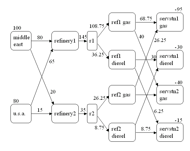
Notice that, in the solution data set (Figure 5.17), the optimal flow through each arc in the network is given in the variable named _FLOW_, and the cost of flow through each arc is given in the variable _FCOST_. As expected, the miminal total cost of the solution found by the interior point algorithm is equal to miminal total cost of the solution found by the simplex algorithm. In this example, the solutions are the same (within several significant digits), but sometimes the solutions can be different.

Figure 5.18: Oil Industry Solution

Interactivity: Network Models: Interior Point Algorithm

PROC NETFLOW can be used interactively. You begin by giving the PROC NETFLOW statement with INTPOINT specified, and you must specify the ARCDATA= data set. The CONDATA= data set must also be specified if the problem has side constraints. If necessary, specify the NODEDATA= data set.

The variable lists should be given next. If you have variables in the input data sets that have special names (for example, a variable in the ARCDATA= data set named _TAIL_ that has tail nodes of arcs as values), it may not be necessary to have many or any variable lists.

So far, this is the same as when the simplex algorithm is used, except the INTPOINT option is specified in the PROC NETFLOW statement. The PRINT, QUIT, SAVE, SHOW, RESET, and RUN statements follow and can be listed in any order. The QUIT statements can be used only once. The others can be used as many times as needed.

The CONOPT and PIVOT statements are not relevant to the interior point algorithm and should not be used.

Use the RESET or SAVE statement to change the name of the output data set. There is only one output data set, the CONOUT= data set. With the RESET statement, you can also indicate the reasons why optimization should stop (for example, you can indicate the maximum number of iterations that can be performed). PROC NETFLOW then has a chance to either execute the next statement, or, if the next statement is one that PROC NETFLOW does not recognize (the next PROC or DATA step in the SAS session), do any allowed optimization and finish. If no new statement has been submitted, you are prompted for one. Some options of the RESET statement enable you to control aspects of the interior point algorithm. Specifying certain values for these options can reduce the time it takes to solve a problem. Note that any of the RESET options can be specified in the PROC NETFLOW statement.

The RUN statement starts optimization. Once the optimization has started, it runs until the optimum is reached. The RUN statement should be specified at most once.

The QUIT statement immediately stops PROC NETFLOW. The SAVE statement has options that allow you to name the output data set; information about the current solution is put in this output data set. Use the SHOW statement if you want to examine the values of options of other statements. Information about the amount of optimization that has been done and the STATUS of the current solution can also be displayed using the SHOW statement.

The PRINT statement makes PROC NETFLOW display parts of the problem. The way the PRINT statements are specified are identical whether the interior point algorithm or the simplex algorithm is used, however there are minor differences in what is displayed for each arc, nonarc variable or constraint coefficient.

PRINT ARCS produces information on all arcs. PRINT SOME_ARCS limits this output to a subset of arcs. There are similar PRINT statements for nonarc variables and constraints:

  
   PRINT NONARCS; 
   PRINT SOME_NONARCS; 
   PRINT CONSTRAINTS; 
   PRINT SOME_CONS;

PRINT CON_ARCS enables you to limit constraint information that is obtained to members of a set of arcs and that have nonzero constraint coefficients in a set of constraints. PRINT CON_NONARCS is the corresponding statement for nonarc variables.

For example, an interactive PROC NETFLOW run might look something like this:

  
   proc netflow 
          intpoint      /* use the Interior Point algorithm */ 
          arcdata=data set 
          other options; 
      variable list specifications;  /* if necessary        */ 
      reset options; 
      print options;                 /* look at problem     */ 
   run;                              /* do the optimization */ 
      print options;    /* look at the optimal solution     */ 
      save options;     /* keep optimal solution            */

If you are interested only in finding the optimal solution, have used SAS variables that have special names in the input data sets, and want to use default settings for everything, then the following statement is all you need.

proc netflow intpoint arcdata= data set ;

Functional Summary: Network Models, Interior Point Algorithm

The following table outlines the options available for the NETFLOW procedure when the interior point algorithm is being used, classified by function. An alphabetical list of options is provided in Dictionary of Options.

Table 5.7: Functional Summary, Network Models

Description	Statement	Option
Input Data Set Options:
arcs input data set	PROC NETFLOW	ARCDATA=
nodes input data set	PROC NETFLOW	NODEDATA=
constraint input data set	PROC NETFLOW	CONDATA=

Output Data Set Option:
constrained solution data set	PROC NETFLOW	CONOUT=

Data Set Read Options:
CONDATA has sparse data format	PROC NETFLOW	SPARSECONDATA
default constraint type	PROC NETFLOW	DEFCONTYPE=
special COLUMN variable value	PROC NETFLOW	TYPEOBS=
special COLUMN variable value	PROC NETFLOW	RHSOBS=
used to interpret arc and nonarc variable names	PROC NETFLOW	NAMECTRL=
no new nonarc variables	PROC NETFLOW	SAME_NONARC_DATA
no nonarc data in ARCDATA	PROC NETFLOW	ARCS_ONLY_ARCDATA
data for an arc found once in ARCDATA	PROC NETFLOW	ARC_SINGLE_OBS
data for a constraint found once in CONDATA	PROC NETFLOW	CON_SINGLE_OBS
data for a coefficient found once in CONDATA	PROC NETFLOW	NON_REPLIC=
data is grouped, exploited during data read	PROC NETFLOW	GROUPED=

Problem Size Specification Options:
approximate number of nodes	PROC NETFLOW	NNODES=
approximate number of arcs	PROC NETFLOW	NARCS=
approximate number of nonarc variables	PROC NETFLOW	NNAS=
approximate number of coefficients	PROC NETFLOW	NCOEFS=
approximate number of constraints	PROC NETFLOW	NCONS=

Network Options:
default arc cost	PROC NETFLOW	DEFCOST=
default arc capacity	PROC NETFLOW	DEFCAPACITY=
default arc lower flow bound	PROC NETFLOW	DEFMINFLOW=
network's only supply node	PROC NETFLOW	SOURCE=
SOURCE's supply capability	PROC NETFLOW	SUPPLY=
network's only demand node	PROC NETFLOW	SINK=
SINK's demand	PROC NETFLOW	DEMAND=
convey excess supply/demand through network	PROC NETFLOW	THRUNET
find maximal flow between SOURCE and SINK	PROC NETFLOW	MAXFLOW
cost of bypass arc for MAXFLOW problem	PROC NETFLOW	BYPASSDIVIDE=
find shortest path from SOURCE to SINK	PROC NETFLOW	SHORTPATH

Memory Control Options:
issue memory usage messages to SAS log	PROC NETFLOW	MEMREP
number of bytes to use for main memory	PROC NETFLOW	BYTES=
proportion of memory for arrays	PROC NETFLOW	COREFACTOR=
maximum bytes for a single array	PROC NETFLOW	MAXARRAYBYTES=

Interior Point Algorithm Options:
use interior point algorithm	PROC NETFLOW	INTPOINT
factorization method	RESET	FACT_METHOD=
allowed amount of dual infeasibility	RESET	TOLDINF=
allowed amount of primal infeasibility	RESET	TOLPINF=
allowed total amount of dual infeasibility	RESET	TOLTOTDINF=
allowed total amount of primal infeasibility	RESET	TOLTOTPINF=
cut-off tolerance for Cholesky factorization	RESET	CHOLTINYTOL=
density threshold for Cholesky processing	RESET	DENSETHR=
step-length multiplier	RESET	PDSTEPMULT=
preprocessing type	RESET	PRSLTYPE=
print optimization progress on SAS log	RESET	PRINTLEVEL2=
write optimization time to SAS log	RESET	OPTIM_TIMER

Interior Point Stopping Criteria Options:
maximum number of interior point iterations	RESET	MAXITERB=
primal-dual (duality) gap tolerance	RESET	PDGAPTOL=
stop because of complementarity	RESET	STOP_C=
stop because of duality gap	RESET	STOP_DG=
stop because of ${infeas}_b$	RESET	STOP_IB=
stop because of ${infeas}_c$	RESET	STOP_IC=
stop because of ${infeas}_d$	RESET	STOP_ID=
stop because of complementarity	RESET	AND_STOP_C=
stop because of duality gap	RESET	AND_STOP_DG=
stop because of ${infeas}_b$	RESET	AND_STOP_IB=
stop because of ${infeas}_c$	RESET	AND_STOP_IC=
stop because of ${infeas}_d$	RESET	AND_STOP_ID=
stop because of complementarity	RESET	KEEPGOING_C=
stop because of duality gap	RESET	KEEPGOING_DG=
stop because of ${infeas}_b$	RESET	KEEPGOING_IB=
stop because of ${infeas}_c$	RESET	KEEPGOING_IC=
stop because of ${infeas}_d$	RESET	KEEPGOING_ID=
stop because of complementarity	RESET	AND_KEEPGOING_C=
stop because of duality gap	RESET	AND_KEEPGOING_DG=
stop because of ${infeas}_b$	RESET	AND_KEEPGOING_IB=
stop because of ${infeas}_c$	RESET	AND_KEEPGOING_IC=
stop because of ${infeas}_d$	RESET	AND_KEEPGOING_ID=

PRINT Statement Options:
display everything	PRINT	PROBLEM
display arc information	PRINT	ARCS
display nonarc variable information	PRINT	NONARCS
display variable information	PRINT	VARIABLES
display constraint information	PRINT	CONSTRAINTS
display information for some arcs	PRINT	SOME_ARCS
display information for some nonarc variables	PRINT	SOME_NONARCS
display information for some variables	PRINT	SOME_VARIABLES
display information for some constraints	PRINT	SOME_CONS
display information for some constraints associated with some arcs	PRINT	CON_ARCS
display information for some constraints associated with some nonarc variables	PRINT	CON_NONARCS
display information for some constraints associated with some variables	PRINT	CON_VARIABLES

PRINT Statement Qualifiers:
produce a short report	PRINT	/ SHORT
produce a long report	PRINT	/ LONG
display arcs/variables with zero flow/value	PRINT	/ ZERO
display arcs/variables with nonzero flow/value	PRINT	/ NONZERO

SHOW Statement Options:
show problem, optimization status	SHOW	STATUS
show network model parameters	SHOW	NETSTMT
show data sets that have been or will be created	SHOW	DATASETS

Miscellaneous Options:
infinity value	PROC NETFLOW	INFINITY=
scale constraint row, nonarc variable column coefficients, or both	PROC NETFLOW	SCALE=
maximization instead of minimization	PROC NETFLOW	MAXIMIZE

Dictionary of Options: Network Models, Interior Point Algorithm

AND_KEEPGOING_C=	AND_KEEPGOING_DG=	AND_KEEPGOING_IB=
AND_KEEPGOING_IC=	AND_KEEPGOING_ID=	AND_STOP_C=
AND_STOP_DG=	AND_STOP_IB=	AND_STOP_IC=
AND_STOP_ID=	ARCDATA=	ARCS
ARCS_ONLY_ARCDATA	ARC_SINGLE_OBS	BYPASSDIVIDE=
BYTES=	CAPACITY Statement	CHOLTINYTOL=
COEF Statement	COLUMN Statement	CONDATA=
CONOUT=	CONSTRAINTS	CON_ARCS
CON_NONARCS	CON_SINGLE_OBS	CON_VARIABLES
COREFACTOR=	COST Statement	DEFCAPACITY=
DEFCONTYPE=	DEFCOST=	DEFMINFLOW=
DEMAND Statement	DEMAND=	DENSETHR=
GROUPED=	HEADNODE Statement	ID Statement
INFINITY=	INTPOINT	KEEPGOING_C=
KEEPGOING_DG=	KEEPGOING_IB=	KEEPGOING_IC=
KEEPGOING_ID=	LO Statement	MAXARRAYBYTES=
MAXFLOW	MAXIMIZE	MAXITERB=
MEMREP	NAME Statement	NAMECTRL=
NARCS=	NCOEFS=	NCONS=
NNAS=	NNODES=	NODE Statement
NODEDATA=	NONARCS	NON_REPLIC=
PDGAPTOL=	PDSTEPMULT=	PRINT Statement
PRINTLEVEL2=	PROBLEM	PRSLTYPE=
QUIT Statement	RESET Statement	RHS Statement
RHSOBS=	ROW Statement	RUN Statement
SAME_NONARC_DATA	SAVE Statement	SCALE=
SHOW Statement	SHORTPATH	SINK=
SOME_ARCS	SOME_CONS	SOME_NONARCS
SOME_VARIABLES	SOURCE=	SPARSECONDATA
STOP_C=	STOP_DG=	STOP_IB=
STOP_IC=	STOP_ID=	SUPDEM Statement
SUPPLY Statement	SUPPLY=	TAILNODE Statement
THRUNET	TOLDINF=	TOLPINF=
TOLTOTDINF=	TOLTOTPINF=	TYPE Statement
TYPEOBS=	VAR Statement	VARIABLES
VERBOSE=

Top of Page