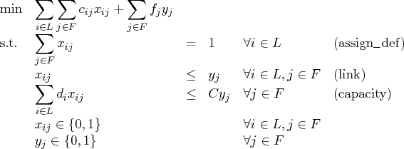
The Mixed Integer Linear Programming Solver

Example 9.3: Facility Location

Consider the classic facility location problem. Given a set l of customer locations and a set f of candidate facility sites, you must decide which sites to build facilities on and assign coverage of customer demand to these sites so as to minimize cost. All customer demand d_i must be satisfied, and each facility has a demand capacity limit c. The total cost is the sum of the distances c_{ij} between facility j and its assigned customer i, plus a fixed charge f_j for building a facility at site j. Let y_j = 1 represent choosing site j to build a facility, and 0 otherwise. Also, let x_{ij} = 1 represent the assignment of customer i to facility j, and 0 otherwise. This model can be formulated as the following integer linear program:

\min & \displaystyle\sum_{i \in l} \displaystyle\sum_{j \in f} c_{ij} x_{ij}    +...   ...\} & & & \forall i \in l, j \in f \    & y_{j} \in \{0,1\} & & & \forall j \in f

Constraint (assign_def) ensures that each customer is assigned to exactly one site. Constraint (link) forces a facility to be built if any customer has been assigned to that facility. Finally, constraint (capacity) enforces the capacity limit at each site.

Let us also consider a variation of this same problem where there is no cost for building a facility. This problem is typically easier to solve than the original problem. For this variant, let the objective be

\min & \displaystyle\sum_{i \in l} \displaystyle\sum_{j \in f} c_{ij} x_{ij}

First, let us construct a random instance of this problem by using the following DATA steps:

    %let NumCustomers  = 50;
    %let NumSites      = 10; 
    %let SiteCapacity  = 35;
    %let MaxDemand     = 10; 
    %let xmax          = 200;
    %let ymax          = 100; 
    %let seed          = 938; 
                                                                                                                                         
    /* generate random customer locations */                                                                                             
    data cdata(drop=i);                                                                                                                  
       length name $8;                                                                                                                   
       do i = 1 to &NumCustomers;                                                                                                        
          name = compress('C'||put(i,best.));                                                                                            
          x = ranuni(&seed) * &xmax;                                                                                                     
          y = ranuni(&seed) * &ymax;                                                                                                     
          demand = ranuni(&seed) * &MaxDemand;                                                                                           
          output;                                                                                                                        
       end;                                                                                                                              
    run;                                                                                                                                 
                                                                                                                                         
    /* generate random site locations and fixed charge */                                                                                
    data sdata(drop=i);                                                                                                                  
       length name $8;                                                                                                                   
       do i = 1 to &NumSites;                                                                                                            
          name = compress('SITE'||put(i,best.));                                                                                         
          x = ranuni(&seed) * &xmax;                                                                                                     
          y = ranuni(&seed) * &ymax;                                                                                                     
          fixed_charge = 30 * (abs(&xmax/2-x) + abs(&ymax/2-y));                                                                
          output;                                                                                                                        
       end;                                                                                                                              
    run;
 

In the following PROC OPTMODEL code, we first generate and solve the model with the no-fixed-charge variant of the cost function. Next, we solve the fixed-charge model. Note that the solution to the model with no fixed charge is feasible for the fixed-charge model and should provide a good starting point for the MILP solver. We use the PRIMALIN option to provide an incumbent solution (warm start).

    proc optmodel;
        set <str> CUSTOMERS;
        set <str> SITES;
 
        /* x and y coordinates of CUSTOMERS and SITES */
        num x {CUSTOMERS union SITES};
        num y {CUSTOMERS union SITES};
        num demand {CUSTOMERS};
        num fixed_charge {SITES};
 
        /* distance from customer i to site j */
        num dist {i in CUSTOMERS, j in SITES}
            = sqrt((x[i] - x[j])^2 + (y[i] - y[j])^2);
 
        read data cdata into CUSTOMERS=[name] x y demand;
        read data sdata into SITES=[name] x y fixed_charge;
 
        var Assign {CUSTOMERS, SITES} binary;
        var Build {SITES} binary;
 
        min CostNoFixedCharge
            = sum {i in CUSTOMERS, j in SITES} dist[i,j] * Assign[i,j];
        min CostFixedCharge
            = CostNoFixedCharge + sum {j in SITES} fixed_charge[j] * Build[j];
 
        /* each customer assigned to exactly one site */
        con assign_def {i in CUSTOMERS}:
           sum {j in SITES} Assign[i,j] = 1;
 
        /* if customer i assigned to site j, then facility must be built at j */
        con link {i in CUSTOMERS, j in SITES}:
            Assign[i,j] <= Build[j];
 
        /* each site can handle at most &SiteCapacity demand */
        con capacity {j in SITES}:
            sum {i in CUSTOMERS} demand[i] * Assign[i,j] <= &SiteCapacity * Build[j];
 
        /* solve the MILP with no fixed charges */
        solve obj CostNoFixedCharge with milp / printfreq = 500;
 
        /* clean up the solution */
        for {i in CUSTOMERS, j in SITES} Assign[i,j] = round(Assign[i,j]);
        for {j in SITES} Build[j] = round(Build[j]);
 
        call symput('varcostNo',put(CostNoFixedCharge,6.1));
 
        /* create a data set for use by GPLOT */
        create data CostNoFixedCharge_Data from
            [customer site]={i in CUSTOMERS, j in SITES: Assign[i,j] = 1}
            xi=x[i] yi=y[i] xj=x[j] yj=y[j];
 
        /* solve the MILP, with fixed charges with warm start */
        solve obj CostFixedCharge with milp / primalin printfreq = 500;
 
        /* clean up the solution */
        for {i in CUSTOMERS, j in SITES} Assign[i,j] = round(Assign[i,j]);
        for {j in SITES} Build[j] = round(Build[j]);
 
        num varcost = sum {i in CUSTOMERS, j in SITES} dist[i,j] * Assign[i,j].sol;
        num fixcost = sum {j in SITES} fixed_charge[j] * Build[j].sol;
        call symput('varcost', put(varcost,6.1));
        call symput('fixcost', put(fixcost,5.1));
        call symput('totalcost', put(CostFixedCharge,6.1));
 
        /* create a data set for use by GPLOT */
        create data CostFixedCharge_Data from
            [customer site]={i in CUSTOMERS, j in SITES: Assign[i,j] = 1}
            xi=x[i] yi=y[i] xj=x[j] yj=y[j];
     quit;
 

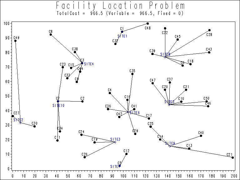
The information printed in the log for the no-fixed-charge model is displayed in Output 9.3.1.

Output 9.3.1: OPTMODEL Log for Facility Location with No Fixed Charges
NOTE: The problem has 510 variables (0 free, 0 fixed).                           
NOTE: The problem has 510 binary and 0 integer variables.                        
NOTE: The problem has 560 linear constraints (510 LE, 50 EQ, 0 GE, 0 range).     
NOTE: The problem has 2010 linear constraint coefficients.                       
NOTE: The problem has 0 nonlinear constraints (0 LE, 0 EQ, 0 GE, 0 range).       
NOTE: The OPTMILP presolver value AUTOMATIC is applied.                          
NOTE: The OPTMILP presolver removed 10 variables and 500 constraints.            
NOTE: The OPTMILP presolver removed 1010 constraint coefficients.                
NOTE: The OPTMILP presolver modified 0 constraint coefficients.                  
NOTE: The presolved problem has 500 variables, 60 constraints, and 1000          
      constraint coefficients.                                                   
NOTE: The MIXED INTEGER LINEAR solver is called.                                 
          Node  Active    Sols    BestInteger      BestBound      Gap    Time    
             0       1       0              .    961.2403449        .       0    
             0       1       2    966.4832160    966.4832160    0.00%       0    
             0       0       2    966.4832160              .    0.00%       0    
NOTE: OPTMILP added 2 cuts with 94 cut coefficients at the root.                 
NOTE: Optimal.                                                                   
NOTE: Objective = 966.483216.                                                    


The results from the warm start approach are shown in Output 9.3.2.

Output 9.3.2: OPTMODEL Log for Facility Location with Fixed Charges, Using Warm Start
NOTE: The problem has 510 variables (0 free, 0 fixed).                           
NOTE: The problem has 510 binary and 0 integer variables.                        
NOTE: The problem has 560 linear constraints (510 LE, 50 EQ, 0 GE, 0 range).     
NOTE: The problem has 2010 linear constraint coefficients.                       
NOTE: The problem has 0 nonlinear constraints (0 LE, 0 EQ, 0 GE, 0 range).       
NOTE: The OPTMILP presolver value AUTOMATIC is applied.                          
NOTE: The OPTMILP presolver removed 0 variables and 0 constraints.               
NOTE: The OPTMILP presolver removed 0 constraint coefficients.                   
NOTE: The OPTMILP presolver modified 0 constraint coefficients.                  
NOTE: The presolved problem has 510 variables, 560 constraints, and 2010         
      constraint coefficients.                                                   
NOTE: The MIXED INTEGER LINEAR solver is called.                                 
          Node  Active    Sols    BestInteger      BestBound      Gap    Time    
             0       1       1  18157.3952518   9946.2514269   82.56%       0    
             0       1       1  18157.3952518   9959.5657588   82.31%       0    
             0       1       1  18157.3952518   9970.3344501   82.11%       0    
             0       1       1  18157.3952518   9974.5475193   82.04%       0    
             0       1       2  11008.3952748   9974.9124195   10.36%       0    
             0       1       2  11008.3952748   9974.9216211   10.36%       0    
             0       1       2  11008.3952748   9975.7667099   10.35%       0    
NOTE: OPTMILP added 16 cuts with 474 cut coefficients at the root.               
             1       2       4  10956.3809482   9975.7667099    9.83%       0    
            21      18       5  10953.9474016   9975.7667099    9.81%       1    
           500     234       5  10953.9474016  10167.0143000    7.74%       7    
          1000     282       5  10953.9474016  10236.9627027    7.00%      16    
          1500     227       5  10953.9474016  10362.9374094    5.70%      23    
          2000      60       5  10953.9474016  10538.2261872    3.94%      30    
          2500     143       5  10953.9474016  10946.0479172    0.07%      35    
          2516     151       6  10952.5054871  10946.1783640    0.06%      35    
          2518     152       7  10952.5054818  10946.1783640    0.06%      35    
          2537      78       8  10948.4603468  10946.3393374    0.02%      35    
          2545      86       9  10948.4603465  10946.3393374    0.02%      35    
          2630      34      10  10948.4603465  10947.4938478    0.01%      36    
NOTE: Optimal within relative gap.                                               
NOTE: Objective = 10948.4603.                                                    


The following two SAS programs produce a plot of the solutions for both variants of the model, using data sets produced by PROC OPTMODEL.

    title1 "Facility Location Problem";                                                                                                 
    title2 "TotalCost = &varcostNo (Variable = &varcostNo, Fixed = 0)";                                                               
    data csdata;                                                                                                                        
        set cdata(rename=(y=cy)) sdata(rename=(y=sy));                                                                                  
    run;                                                                                                                                
    /* create Annotate data set to draw line between customer and assigned site */                                                      
    %annomac;                                                                                                                           
    data anno(drop=xi yi xj yj);                                                                                                        
       %SYSTEM(2, 2, 2);                                                                                                               
       set CostNoFixedCharge_Data(keep=xi yi xj yj);                                                                                    
       %LINE(xi, yi, xj, yj, *, 1, 1);                                                                                                  
    run;                                                                                                                                
    proc gplot data=csdata anno=anno;                                                                                                   
       axis1 label=none order=(0 to &xmax by 10);                                                                                       
       axis2 label=none order=(0 to &ymax by 10);                                                                                       
       symbol1 value=dot interpol=none                                                                                                  
          pointlabel=("#name" nodropcollisions height=1) cv=black;                                                                   
       symbol2 value=diamond interpol=none                                                                                              
          pointlabel=("#name" nodropcollisions color=blue height=1) cv=blue;                                                                    
       plot cy*x sy*x / overlay haxis=axis1 vaxis=axis2;                                                                                
    run;
    quit;
 

The output of the first program is shown in Output 9.3.3.

Output 9.3.3: Solution Plot for Facility Location with No Fixed Charges
milpexfacloc4plot.gif (11586 bytes)


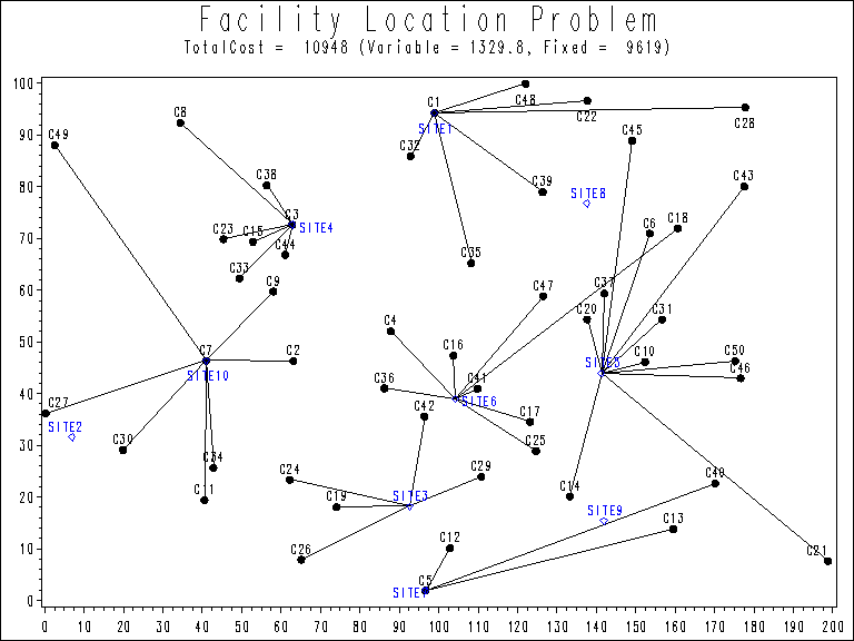
The output of the second program is shown in Output 9.3.4.

    title1 "Facility Location Problem";                                                                                                 
    title2 "TotalCost = &totalcost (Variable = &varcost, Fixed = &fixcost)";                                                        
    /* create Annotate data set to draw line between customer and assigned site */                                                      
    data anno(drop=xi yi xj yj);                                                                                                        
       %SYSTEM(2, 2, 2);                                                                                                                
       set CostFixedCharge_Data(keep=xi yi xj yj);                                                                                      
       %LINE(xi, yi, xj, yj, *, 1, 1);                                                                                                  
    run;
    proc gplot data=csdata anno=anno;                                                                                                   
       axis1 label=none order=(0 to &xmax by 10);                                                                                       
       axis2 label=none order=(0 to &ymax by 10);                                                                                       
       symbol1 value=dot interpol=none                                                                                                  
          pointlabel=("#name" nodropcollisions height=1) cv=black;                                                                    
       symbol2 value=diamond interpol=none                                                                                              
          pointlabel=("#name" nodropcollisions color=blue height=1) cv=blue;                                                                    
       plot cy*x sy*x / overlay haxis=axis1 vaxis=axis2;                                                                                
    run;
    quit;
 

Output 9.3.4: Solution Plot for Facility Location with Fixed Charges
milpexfacloc5plot.gif (12546 bytes)


The economic trade-off for the fixed-charge model forces us to build fewer sites and push more demand to each site.

It is possible to expedite the solution of the fixed-charge facility location problem by choosing appropriate branching priorities for the decision variables. Recall that for each site j, the value of the variable y_j determines whether or not a facility is built on that site. Suppose you decide to branch on the variables y_j before the variables x_{ij}. You can set a higher branching priority for y_j by using the .priority suffix for the Build variables in PROC OPTMODEL, as follows:

  
 for{j in SITES} Build[j].priority=10;
 

Setting higher branching priorities for certain variables is not guaranteed to speed up the MILP solver, but it can be helpful in some instances. The following program creates and solves an instance of the facility location problem in which giving higher priority to y_j causes the MILP solver to find the optimal solution more quickly. We use the PRINTFREQ= option to abbreviate the node log.

     %let NumCustomers  = 45;    
     %let NumSites      = 8;    
     %let SiteCapacity  = 35;    
     %let MaxDemand     = 10;    
     %let xmax          = 200;    
     %let ymax          = 100;    
     %let seed          = 2345;
 
     /* generate random customer locations */
     data cdata(drop=i);
        length name $8;
        do i = 1 to &NumCustomers;
           name = compress('C'||put(i,best.));
           x = ranuni(&seed) * &xmax;
           y = ranuni(&seed) * &ymax;
           demand = ranuni(&seed) * &MaxDemand;
           output;
        end;
     run;
 
     /* generate random site locations and fixed charge */
     data sdata(drop=i);
        length name $8;
        do i = 1 to &NumSites;
           name = compress('SITE'||put(i,best.));
           x = ranuni(&seed) * &xmax;
           y = ranuni(&seed) * &ymax;
           fixed_charge = (abs(&xmax/2-x) + abs(&ymax/2-y)) / 2;
           output;
        end;
     run;
 

    proc optmodel; 
                                                                                                                                                                                                                               
       set <str> CUSTOMERS;
       set <str> SITES;
 
       /* x and y coordinates of CUSTOMERS and SITES */
       num x {CUSTOMERS union SITES};
       num y {CUSTOMERS union SITES};
       num demand {CUSTOMERS};
       num fixed_charge {SITES};
           
       /* distance from customer i to site j */
       num dist {i in CUSTOMERS, j in SITES} 
           = sqrt((x[i] - x[j])^2 + (y[i] - y[j])^2);
 
       read data cdata into CUSTOMERS=[name] x y demand;
       read data sdata into SITES=[name] x y fixed_charge;
 
       var Assign {CUSTOMERS, SITES} binary;
       var Build {SITES} binary;
 
       min CostFixedCharge   
           = sum {i in CUSTOMERS, j in SITES} dist[i,j] * Assign[i,j] 
             + sum {j in SITES} fixed_charge[j] * Build[j];
       
       /* each customer assigned to exactly one site */
       con assign_def {i in CUSTOMERS}:
          sum {j in SITES} Assign[i,j] = 1;
 
       /* if customer i assigned to site j, then facility must be built at j */
       con link {i in CUSTOMERS, j in SITES}:
           Assign[i,j] <= Build[j];
 
       /* each site can handle at most &SiteCapacity demand */
       con capacity {j in SITES}:
           sum {i in CUSTOMERS} demand[i] * Assign[i,j] <= &SiteCapacity * Build[j];
 
       /* assign priority to Build variables (y) */
       for{j in SITES} Build[j].priority=10;
 
       /* solve the MILP with fixed charges, using branching priorities */
       solve obj CostFixedCharge with milp / printfreq=1000;
       
    quit;
 

The resulting output is shown in Output 9.3.5.

Output 9.3.5: PROC OPTMODEL Log for Facility Location with Branching Priorities
NOTE: There were 45 observations read from the data set WORK.CDATA.              
NOTE: There were 8 observations read from the data set WORK.SDATA.               
NOTE: The problem has 368 variables (0 free, 0 fixed).                           
NOTE: The problem has 368 binary and 0 integer variables.                        
NOTE: The problem has 413 linear constraints (368 LE, 45 EQ, 0 GE, 0 range).     
NOTE: The problem has 1448 linear constraint coefficients.                       
NOTE: The problem has 0 nonlinear constraints (0 LE, 0 EQ, 0 GE, 0 range).       
NOTE: The OPTMILP presolver value AUTOMATIC is applied.                          
NOTE: The OPTMILP presolver removed 0 variables and 0 constraints.               
NOTE: The OPTMILP presolver removed 0 constraint coefficients.                   
NOTE: The OPTMILP presolver modified 0 constraint coefficients.                  
NOTE: The presolved problem has 368 variables, 413 constraints, and 1448         
      constraint coefficients.                                                   
NOTE: The MIXED INTEGER LINEAR solver is called.                                 
          Node  Active    Sols    BestInteger      BestBound      Gap    Time    
             0       1       0              .   1727.0208789        .       0    
             0       1       0              .   1742.9508521        .       0    
             0       1       0              .   1752.2235082        .       0    
             0       1       0              .   1774.0288243        .       0    
             0       1       0              .   1775.9603081        .       0    
             0       1       0              .   1778.5118008        .       0    
             0       1       0              .   1780.4356268        .       0    
             0       1       0              .   1782.2847353        .       0    
NOTE: OPTMILP added 31 cuts with 819 cut coefficients at the root.               
             1       2       2   1897.2016698   1782.2847353    6.45%       0    
             3       4       4   1845.6411894   1782.2847353    3.55%       1    
             6       7       5   1836.6772083   1782.2847353    3.05%       1    
             7       8       6   1836.6772076   1782.2847353    3.05%       1    
            20      21       7   1823.4483963   1782.2847353    2.31%       1    
           820     429       8   1823.3287600   1811.3016072    0.66%       6    
          1000     429       8   1823.3287600   1812.5380697    0.60%       8    
          1513     235       9   1819.9124342   1817.5781767    0.13%      11    
          1789      17       9   1819.9124342   1819.7319707    0.01%      14    
NOTE: Optimal within relative gap.                                               
NOTE: Objective = 1819.91243.                                                    


The output in Output 9.3.6 is generated by running the same program without the line that assigns higher branching priorities to the Build variables. We again use the PRINTFREQ= option to abbreviate the node log.

Output 9.3.6: PROC OPTMODEL Log for Facility Location without Branching Priorities
NOTE: There were 45 observations read from the data set WORK.CDATA.              
NOTE: There were 8 observations read from the data set WORK.SDATA.               
NOTE: The problem has 368 variables (0 free, 0 fixed).                           
NOTE: The problem has 368 binary and 0 integer variables.                        
NOTE: The problem has 413 linear constraints (368 LE, 45 EQ, 0 GE, 0 range).     
NOTE: The problem has 1448 linear constraint coefficients.                       
NOTE: The problem has 0 nonlinear constraints (0 LE, 0 EQ, 0 GE, 0 range).       
NOTE: The OPTMILP presolver value AUTOMATIC is applied.                          
NOTE: The OPTMILP presolver removed 0 variables and 0 constraints.               
NOTE: The OPTMILP presolver removed 0 constraint coefficients.                   
NOTE: The OPTMILP presolver modified 0 constraint coefficients.                  
NOTE: The presolved problem has 368 variables, 413 constraints, and 1448         
      constraint coefficients.                                                   
NOTE: The MIXED INTEGER LINEAR solver is called.                                 
          Node  Active    Sols    BestInteger      BestBound      Gap    Time    
             0       1       0              .   1727.0208789        .       0    
             0       1       0              .   1742.9508521        .       0    
             0       1       0              .   1752.2235082        .       0    
             0       1       0              .   1774.0288243        .       0    
             0       1       0              .   1775.9603081        .       0    
             0       1       0              .   1778.5118008        .       0    
             0       1       0              .   1780.4356268        .       0    
             0       1       0              .   1782.2847353        .       0    
NOTE: OPTMILP added 31 cuts with 819 cut coefficients at the root.               
             1       2       2   1845.6411909   1798.0236457    2.65%       1    
            99      92       3   1830.2464078   1798.1088996    1.79%       1    
           130     113       4   1828.3829705   1798.1114430    1.68%       2    
           178     148       5   1826.5738687   1801.3003022    1.40%       3    
           252     203       6   1825.5361998   1802.8877583    1.26%       3    
          1651     779       7   1822.8640271   1813.2363990    0.53%      10    
          2302     668       8   1821.5115364   1816.1164144    0.30%      15    
          2362     466       9   1819.9124342   1816.3899402    0.19%      15    
          2939      17       9   1819.9124342   1819.7324195    0.01%      21    
NOTE: Optimal within relative gap.                                               
NOTE: Objective = 1819.91243.                                                    


By comparing Output 9.3.5 and Output 9.3.6 you can see that in this instance, increasing the branching priorities of the Build variables results in computational savings.

Previous Page | Next Page | Top of Page