| The Linear Programming Solver |
Example 8.3: Two-Person Zero-Sum Game
Consider a two-person zero-sum game (where one person wins what the other person loses). The players make moves simultaneously, and each has a choice of actions. There is a payoff matrix that indicates the amount one player gives to the other under each combination of actions:
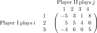
If player I makes move ![]() and player II makes move
and player II makes move ![]() , then player I wins (and player II loses)
, then player I wins (and player II loses) ![]() . What is the best strategy for the two players to adopt? This example is simple enough to be analyzed from observation. Suppose player I plays 1 or 3; the best response of player II is to play 1. In both cases, player I loses and player II wins. So the best action for player I is to play 2. In this case, the best response for player II is to play 3, which minimizes the loss. In this case, (2, 3) is a pure-strategy Nash equilibrium in this game.
. What is the best strategy for the two players to adopt? This example is simple enough to be analyzed from observation. Suppose player I plays 1 or 3; the best response of player II is to play 1. In both cases, player I loses and player II wins. So the best action for player I is to play 2. In this case, the best response for player II is to play 3, which minimizes the loss. In this case, (2, 3) is a pure-strategy Nash equilibrium in this game.
For illustration, consider the following mixed strategy case. Assume that player I selects ![]() with probability
with probability ![]() , and player II selects
, and player II selects ![]() with probability
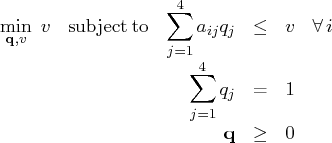
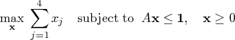
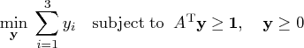
with probability ![]() . Consider player II's problem of minimizing the maximum expected payout:
. Consider player II's problem of minimizing the maximum expected payout:
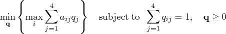
This is equivalent to
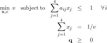
We can transform the problem into a more standard format by making a simple change of variables: ![]() . The preceding LP formulation now becomes
. The preceding LP formulation now becomes
    proc optmodel;
       num a{1..3, 1..4}=[-5 3 1 8
                           5 5 4 6
                          -4 6 0 5];
       var x{1..4} >= 0;
       max f = sum{i in 1..4}x[i];
       con c{i in 1..3}: sum{j in 1..4}a[i,j]*x[j] <= 1;
       solve with lp / solver = ps presolver = none printfreq = 1;
       print x;
       print c.dual;
    quit;
The optimal solution is displayed in Output 8.3.1.
Output 8.3.1: Optimal Solutions to the Two-Person Zero-Sum GameThe optimal solution ![]() with an optimal value of 0.25. Therefore the optimal strategy for player II is
with an optimal value of 0.25. Therefore the optimal strategy for player II is ![]() . You can check the optimal solution of the dual problem by using the constraint suffix ".dual". So
. You can check the optimal solution of the dual problem by using the constraint suffix ".dual". So ![]() and player I's optimal strategy is (0, 1, 0). The solution is consistent with our intuition from observation.
and player I's optimal strategy is (0, 1, 0). The solution is consistent with our intuition from observation.
Copyright © 2008 by SAS Institute Inc., Cary, NC, USA. All rights reserved.