The Interior Point Nonlinear Programming Solver -- Experimental

Getting Started

Consider the following simple example of a nonlinear optimization problem:

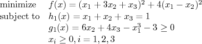
$\displaystyle\mathop{\rm minimize}& f(x) = ( x_{1}+3x_{2}+x_{3} )^2 + 4( x_{1}-x... ... & g_{1}(x) = 6x_{2} + 4x_{3} - x_{1}^3 -3 \ge 0 \ & x_{i} \ge 0, i = 1, 2 ,3$

The problem consists of a quadratic objective function, a linear equality, and a nonlinear inequality constraint. We are interested in finding a local minimum, starting from the point

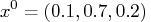
. To achieve this, we write the following SAS code:

    proc optmodel;
       var x{1..3} >= 0;
       minimize obj = ( x[1] + 3*x[2] + x[3] )**2 + 4*(x[1] - x[2])**2;
    
       con constr1: sum{i in 1..3}x[i] = 1;
       con constr2: 6*x[2] + 4*x[3] - x[1]**3 -3 >= 0;
    
       /* starting point */
       x[1] = 0.1;
       x[2] = 0.7;
       x[3] = 0.2;
    
       solve with IPNLP;
       print x;
    quit;

The SAS output displays a detailed summary of the problem, together with the status of the solver at termination, the total number of iterations required, and the value of the objective function at the local minimum. The summary and the optimal solution are shown in Output 7.1.

The OPTMODEL Procedure

Problem Summary
Objective Sense	Minimization
Objective Function	obj
Objective Type	Quadratic

Number of Variables	3
Bounded Above	0
Bounded Below	3
Bounded Below and Above	0
Free	0
Fixed	0

Number of Constraints	2
Linear LE (<=)	0
Linear EQ (=)	1
Linear GE (>=)	0
Linear Range	0
Nonlinear LE (<=)	0
Nonlinear EQ (=)	0
Nonlinear GE (>=)	1
Nonlinear Range	0

The OPTMODEL Procedure

Solution Summary
Solver	IPNLP
Objective Function	obj
Solution Status	Optimal
Objective Value	1.0000053879
Iterations	21

Infeasibility	2.810568E-10
Optimality Error	7.8706805E-7

[1]	x
1	0.00071696
2	0.00000083
3	0.99928221

Figure 7.1: Problem Summary and the Optimal Solution

The SAS log shown in Output 7.2 displays a brief summary of the problem being solved, followed by the iterations generated by the solver.


NOTE: The problem has 3 variables (0 free, 0 fixed).
NOTE: The problem has 1 linear constraints (0 LE, 1 EQ, 0 GE, 0 range).
NOTE: The problem has 3 linear constraint coefficients.
NOTE: The problem has 1 nonlinear constraints (0 LE, 0 EQ, 1 GE, 0 range).
NOTE: This is an experimental version of the IPNLP solver.
NOTE: Using analytic derivatives for objective.
NOTE: Using analytic derivatives for nonlinear constraints.
NOTE: The IPNLP solver is called.
Objective Optimality
Iter Value Infeasibility Error
0 25.00000000 2.00000000 70.04792090
1 8.25327051 1.60939368 35.77834471
2 6.39960188 1.23484604 20.13229803
3 2.04185087 0.07936183 3.03960094
4 1.54274807 0.00397738 1.06189744
5 1.28365293 0.00020216 0.43781371
6 1.14816541 0.00004932 0.19807160
7 1.07829315 0.00007323 0.11097627
8 1.04065865 0.00007384 0.08008765
9 1.02071978 0.00005144 0.02705360
10 1.01052389 0.00001978 0.00810753
11 1.00533187 0.00000746 0.00340008
12 1.00269340 0.00000282 0.00146226
13 1.00135663 0.00000104 0.00062682
14 1.00068185 0.0000003814609 0.00027023
15 1.00034218 0.0000001378457 0.00011693
16 1.00017153 0.0000000494663 0.00005071
17 1.00008592 0.0000000176688 0.00002202
18 1.00004302 0.0000000062912 0.00000957
19 1.00002153 0.0000000022353 0.00000416
20 1.00001077 0.0000000007930 0.00000181
21 1.00000539 0.0000000002811 0.0000007870680
NOTE: Converged.
NOTE: Objective = 1.00000539.

Figure 7.2: Progress of the Algorithm as Shown in the Log

Top of Page