The NLPC Nonlinear Optimization Solver

Introductory Examples

The following introductory examples illustrate how to get started using the NLPC solver and also provide basic information about the use of PROC OPTMODEL.

An Unconstrained Problem

Consider the following example of minimizing the Rosenbrock function (Rosenbrock 1960):

where . The minimum function value is at . Note that this problem has no constraints.

The following PROC OPTMODEL statements can be used to solve this problem:

    proc optmodel;
       number a = 100;
       var x{1..2};
       min f = a*(x[2] - x[1]^2)^2 + (1 - x[1])^2;
 
       solve with nlpc / tech=newtyp;
       print x;
    quit;
 

The VAR statement declares the decision variables and . The MIN statement identifies the symbol that defines the objective function in terms of and . The TECH=NEWTYP option in the SOLVE statement specifies that the Newton-type method with line search is used to solve this problem. Finally, the PRINT statement is specified to display the solution to this problem.

The output that summarizes the problem characteristics and the solution obtained by the solver are displayed in Figure 10.1. Note that the solution has and , and an objective value very close to .

Problem Summary Objective Sense Minimization Objective Function f Objective Type Nonlinear     Number of Variables 2 Bounded Above 0 Bounded Below 0 Bounded Below and Above 0 Free 2 Fixed 0     Number of Constraints 0 Solution Summary Solver NLPC/Newton-Type Objective Function f Solution Status Optimal Objective Value 6.429583E-18 Iterations 14     Absolute Optimality Error 4.8615356E-8 Relative Optimality Error 4.8615356E-8 Absolute Infeasibility 0 Relative Infeasibility 0 [1] x 1 1 2 1

Figure 10.1: Minimization of the Rosenbrock Function

Bound Constraints on the Decision Variables

Decision variables often have bound constraints of the form

where is the number of decision variables. The bounds on the variables can be specified with the symbols ">=" and "<=" in the VAR statement.

Consider the following bound constrained problem (Hock and Schittkowski 1981, Example 5):

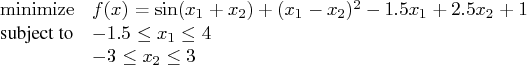
Given a starting point at , there is a local minimum at

with the objective value . This problem can be formulated and solved by the following statements:

    proc optmodel;
       set S = 1..2;
       number lb{S} = [-1.5 -3];
       number ub{S} = [4 3];
       number x0{S} = [0 0];
       var x{i in S} >= lb[i] <= ub[i] init x0[i];
       
       min obj = sin(x[1] + x[2]) + (x[1] - x[2])^2
                   - 1.5*x[1] + 2.5*x[2] + 1;
 
       solve with nlpc / printfreq=1;
       print x;
    quit;
 

The starting point is specified with the keyword INIT in the VAR statement. As usual, the MIN statement identifies the objective function. Since there is no explicit optimization technique specified (using the TECH= option), the NLPC solver uses the trust region method, which is the default algorithm for problems of this size. The PRINTFREQ= option is used to display the iteration log during the optimization process.

In Figure 10.2, the problem is summarized at the top. Then, the details of the iterations are displayed. A message is printed to indicate that the default optimality criteria (ABSOPTTOL=0.001, RELOPTTOL=1.0E-6) were satisfied. (See the section "Optimality Control" for more information.) A summary of the solution shows that the trust region method was used for the optimization and the solution found is optimal. It also shows the optimal objective value and the number of iterations taken to find the solution. The optimal solution is displayed at the end.

Problem Summary Objective Sense Minimization Objective Function obj Objective Type Nonlinear     Number of Variables 2 Bounded Above 0 Bounded Below 0 Bounded Below and Above 2 Free 0 Fixed 0     Number of Constraints 0 Iteration Log: Trust Region Method Iter Function Calls Objective Value Optimality Error Trust Region Radius 0 0 1.0000 1.0000 . 1 2 -1.5758 0.8905 2.231 2 4 -1.8962 0.2414 0.546 3 5 -1.9131 0.0127 0.554 4 6 -1.9132 0.0000521 0.149 5 7 -1.9132 9.061E-10 0.0103 Note: Optimality criteria (ABSOPTTOL=0.001, RELOPTTOL=1E-6) are satisfied. Solution Summary Solver NLPC/Trust Region Objective Function obj Solution Status Optimal Objective Value -1.913222955 Iterations 5     Absolute Optimality Error 9.061385E-10 Relative Optimality Error 9.061385E-10 Absolute Infeasibility 0 Relative Infeasibility 0 [1] x 1 -0.5472 2 -1.5472

Figure 10.2: A Bound Constrained Problem

Linear Constraints on the Decision Variables

More general linear equality or inequality constraints have the form

where is the number of decision variables and is the number of constraints, which can be specified with the CON statement.

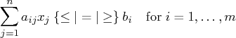
Consider, for example, Rosenbrock's post office problem (Schittkowski 1987, p. 74):

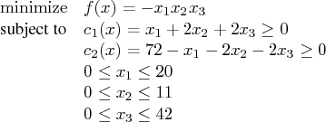
Starting from , you can reach a minimum at , with a corresponding objective value . You can use the following SAS code to formulate and solve this problem:

    proc optmodel;
       number ub{1..3} = [20 11 42];
       var x{i in 1..3} >= 0 <= ub[i] init 10;
       
       min f = -1*x[1]*x[2]*x[3];
       con c1: x[1] + 2*x[2] + 2*x[3] >= 0;
       con c2: 72 - x[1] - 2*x[2] - 2*x[3] >= 0;
       
       solve with nlpc / tech=congra printfreq=1;
       print x;
    quit;
 

As usual, the VAR statement specifies the bounds on the variables, and the starting point; the MIN statement identifies the objective function. In addition, the two CON statements describe the linear constraints and . To solve this problem, select the conjugate gradient optimization technique by using the TECH=CONGRA option. The PRINTFREQ= option is used to display the iteration log.

In Figure 10.3, you can find a problem summary and the iteration log. The solution summary and the solution are printed at the bottom.

Problem Summary Objective Sense Minimization Objective Function f Objective Type Nonlinear     Number of Variables 3 Bounded Above 0 Bounded Below 0 Bounded Below and Above 3 Free 0 Fixed 0     Number of Constraints 2 Linear LE (<=) 0 Linear EQ (=) 0 Linear GE (>=) 2 Linear Range 0 Iteration Log: Conjugate Gradient Method Iter Function Calls Objective Value Optimality Error Step Size Slope of Search Direction Restarts 0 0 -1000 1.0000 . . 0 1 2 -1331 1.0000 0.0100 -30000 0 2 4 -3056 0.2952 0.0468 -29282 1 3 6 -3300 0 0.0455 -6722.2 2 Note: Optimality criteria (ABSOPTTOL=0.001, RELOPTTOL=1E-6) are satisfied. Solution Summary Solver NLPC/Conjugate Gradient Objective Function f Solution Status Optimal Objective Value -3300 Iterations 3     Absolute Optimality Error 0 Relative Optimality Error 0 Absolute Infeasibility 3.552714E-15 Relative Infeasibility 4.866731E-17 [1] x 1 20 2 11 3 15

Figure 10.3: Rosenbrock's Post Office Problem

You can formulate linear constraints in a more compact manner. Consider the following example (Hock and Schittkowski 1981, test example 24):

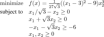
The minimum function value is at . Assume a feasible starting point, .

You can specify this model by using the following PROC OPTMODEL statements:

    proc optmodel;
       number a{1..3, 1..2} = [ .57735     -1
                                     1  1.732
                                    -1 -1.732 ];
       number b{1..3} = [ 0 0 -6 ];
       number x0{1..2} = [ 1 .5 ];
       var x{i in 1..2} >= 0 init x0[i];
       
       min f = ((x[1] - 3)^2 - 9) * x[2]^3 / (27*sqrt(3));
       con cc {i in 1..3}: sum{j in 1..2} a[i,j]*x[j] >= b[i];
 
       solve with nlpc / printfreq=1;
       print x;
    quit;
 

Note that instead of writing three individual linear constraints as in Rosenbrock's post office problem, we use a two-dimensional array to represent the coefficient matrix of the linear constraints and a one-dimensional array for the right-hand side. Consequently, all three linear constraints are represented in a single CON statement. This method is especially useful for larger models and for models in which the constraint coefficients are subject to change.

The output showing the problem summary, the iteration log, the solution summary, and the solution is displayed in Figure 10.4.

Problem Summary Objective Sense Minimization Objective Function f Objective Type Nonlinear     Number of Variables 2 Bounded Above 0 Bounded Below 2 Bounded Below and Above 0 Free 0 Fixed 0     Number of Constraints 3 Linear LE (<=) 0 Linear EQ (=) 0 Linear GE (>=) 3 Linear Range 0 Iteration Log: Trust Region Method Iter Function Calls Objective Value Optimality Error Trust Region Radius 0 0 -0.0134 0.0802 . 1 1 -0.0218 0.0706 1.000 2 7 -1.0000 0 9.166 Note: Optimality criteria (ABSOPTTOL=0.001, RELOPTTOL=1E-6) are satisfied. Solution Summary Solver NLPC/Trust Region Objective Function f Solution Status Optimal Objective Value -1.000043302 Iterations 2     Absolute Optimality Error 0 Relative Optimality Error 0 Absolute Infeasibility 0 Relative Infeasibility 0 [1] x 1 3.0000 2 1.7321

Figure 10.4: A Second Linearly Constrained Problem

Nonlinear Constraints on the Decision Variables

General nonlinear equality or inequality constraints have the form

where is a general nonlinear constraint, which can be specified with the CON statement.

Consider the following nonlinearly constrained problem (Avriel 1976, p. 456):

An initial point is given at . You can use the following SAS code to formulate and solve this problem:

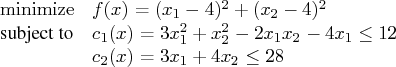
    proc optmodel;
       num x0{1..2} = [2 0];
       var x{i in 1..2} init x0[i];
       
       min f = (x[1] - 4)^2 + (x[2] - 4)^2;
       con c1: 3*x[1]^2 + x[2]^2 - 2*x[1]*x[2] - 4*x[1] <= 12;
       con c2: 3*x[1] + 4*x[2] <= 28;
       
       solve with nlpc / tech=qne printfreq=1;
       print x;
    quit;
 

Note that is a nonlinear constraint and is a linear constraint. Both can be specified by using the CON statement. The PROC OPTMODEL modeling language automatically recognizes types of constraints to which they belong. The experimental quasi-Newton method is requested to solve this problem.

A problem summary is shown in Figure 10.5. Figure 10.6 displays the iteration log. Note that the quasi-Newton method is an infeasible point algorithm; i.e., the iterates remain infeasible to the nonlinear constraints until the optimal solution is found. The column "Maximum Constraint Violation" displays the infeasibility. The solution summary and the solution are shown in Figure 10.7.

Problem Summary Objective Sense Minimization Objective Function f Objective Type Quadratic     Number of Variables 2 Bounded Above 0 Bounded Below 0 Bounded Below and Above 0 Free 2 Fixed 0     Number of Constraints 2 Linear LE (<=) 1 Linear EQ (=) 0 Linear GE (>=) 0 Linear Range 0 Nonlinear LE (<=) 1 Nonlinear EQ (=) 0 Nonlinear GE (>=) 0 Nonlinear Range 0

Figure 10.5: Nonlinearly Constrained Problem: Problem Summary

Iteration Log: Quasi-Newton Method with BFGS Update Iter Function Calls Objective Value Infeasibility Optimality Error Step Size Predicted Function Reduction 0 0 20.0000 0 1.0000 . . 1 1 0.9570 0 1.0275 1.000 1.7256 2 2 0.0942 0.0480 0.1134 1.000 0.0783 3 3 0.1335 0.000538 0.004636 1.000 0.00103 4 4 0.1340 2.9482E-7 0.000336 1.000 5.148E-7 5 5 0.1340 2.1822E-9 2.4734E-6 1.000 4.2E-9 6 6 0.1340 1.159E-13 6.4421E-9 1.000 2.101E-9 Note: Optimality criteria (ABSOPTTOL=0.001, RELOPTTOL=1E-6) are satisfied.

Figure 10.6: Nonlinearly Constrained Problem: Iteration Log

Solution Summary Solver NLPC/Quasi-Newton Objective Function f Solution Status Optimal Objective Value 0.134001789 Iterations 6     Absolute Optimality Error 6.4420693E-9 Relative Optimality Error 6.4420693E-9 Absolute Infeasibility 1.506351E-12 Relative Infeasibility 1.158731E-13 [1] x 1 3.6348 2 3.9748

Figure 10.7: Nonlinearly Constrained Problem: Solution