| The CLP Procedure |
Example 1.2 Scheduling with Alternate Resources
This example shows an interesting job shop scheduling problem illustrating the use of alternative resources. There are 90 jobs (J1–J90) that need to be processed on one of 10 machines (M0–M9). Not every machine can process every job. In addition, certain jobs might also require one of 7 operators (OP0–OP6). As with the machines, not every operator can be assigned to every job. There are no explicit precedence relationships in this example.
The machine and operator requirements for each job are specified within the data set proj by using the following statements.
   /* project specification */
   data proj;
      array v{11} $8. j1-j3 m1-m3 o1-o4 dur;
      input v{*};
      datalines;
   1    .    .    0    1    .    0    1    2    .    1
   2    .    .    0    1    2    0    1    2    .    1
   3    .    .    1    2    3    0    1    2    .    1
   4    5    6    3    4    5    2    3    4    5    1
   7    .    .    6    7    8    5    6    .    .    1
   8    9    .    6    7    8    .    .    .    .    1
   10   .    .    7    8    9    .    .    .    .    1
   11   .    .    1    2    .    0    1    2    3    1
   12   13   14   7    8    9    0    1    2    3    1
   15   16   .    5    6    .    4    5    6    .    1
   17   .    .    3    4    .    4    5    6    .    1
   18   .    .    3    4    .    .    .    .    .    1
   19   .    .    0    1    2    .    .    .    .    1
   20   .    .    0    1    .    .    .    .    .    1
   21   22   .    0    1    .    0    1    2    .    2
   23   .    .    2    .    .    0    1    2    .    2
   24   25   36   8    9    .    .    .    .    .    1
   26   35   75   6    7    .    .    .    .    .    1
   27   34   74   6    7    .    5    6    .    .    1
   28   .    .    4    5    .    5    6    .    .    1
   29   .    .    4    5    .    3    4    .    .    1
   30   .    .    3    .    .    3    4    .    .    1
   31   .    .    3    .    .    3    4    .    .    2
   32   .    .    4    5    .    3    4    .    .    2
   33   .    .    4    5    .    5    6    .    .    2
   37   76   77   8    9    .    .    .    .    .    1
   38   39   .    0    1    .    0    1    .    .    1
   40   .    .    2    .    .    2    .    .    .    1
   41   .    .    6    7    .    6    .    .    .    2
   42   62   82   6    7    .    .    .    .    .    2
   43   44   63   8    9    .    .    .    .    .    2
   45   46   65   0    1    .    4    5    .    .    2
   47   67   .    2    3    .    2    3    .    .    2
   48   68   .    2    3    .    2    3    .    .    1
   49   50   69   4    5    .    0    1    .    .    1
   51   52   .    3    4    .    1    2    .    .    2
   53   .    .    5    6    .    0    .    .    .    2
   54   .    .    5    6    .    6    .    .    .    1
   55   56   57   7    8    9    .    .    .    .    1
   58   59   78   0    1    2    3    4    .    .    1
   60   80   .    0    1    2    5    6    .    .    1
   61   81   .    6    7    .    5    6    .    .    2
   64   83   84   8    9    .    .    .    .    .    2
   66   .    .    0    1    .    4    5    .    .    2
   70   .    .    5    .    .    0    1    .    .    1
   71   .    .    5    .    .    0    1    2    .    2
   72   73   .    3    4    .    0    1    2    .    2
   79   .    .    0    1    2    3    4    .    .    1
   85   .    .    0    .    .    3    .    .    .    1
   86   .    .    1    .    .    4    .    .    .    1
   87   .    .    2    .    .    5    .    .    .    1
   88   .    .    3    .    .    0    .    .    .    1
   89   .    .    4    .    .    1    .    .    .    1
   90   .    .    5    .    .    2    .    .    .    1
   ;
Each row in the datalines section defines a resource requirement for up to three jobs that are identified in the variables j1–j3. The resource requirement associated with each of these jobs is a set of alternates and is defined using the variables m1–m3 and o1–o4.
The variables m1–m3 represent a machine or workstation ID that the job needs to be processed on, and the variables o1–o4 represent an operator ID. The duration of each of the jobs identified in j1–j3 is assumed to be identical and defined using the dur variable. Each of the jobs in a row can be processed on any one of the machines in m1–m3 and requires the assistance of one of the operators in o1–o4 while being processed. In other words, the resource requirement for each job is a conjunction of disjunctive requirements (or alternates). A job requires one of m1–m3 and one of o1–o4 in order to be processed. For example, observation 5 specifies that job number 7 can be processed on either machine 6, 7, or 8 and additionally requires either operator 5 or operator 6 in order to be processed. The next observation indicates that jobs 8 and 9 can also be processed on the same set of machines. However, they do not require any operator assistance.
The ACTIVITY and REQUIRES statements for the CLP procedure are next generated from the data set proj by the following program:
   /* generate the ACTIVITY and REQUIRES statements */
   data _null_;
      set proj end=finish;
      format jobs $32. resources $char128.;
      format acts reqs $char4096.;
      retain acts reqs;
      array v{11} j1-j3 m1-m3 o1-o4 dur;
      jobs=catx(' J',of j1-j3);
      acts=catx(' ',acts,cats('(J',jobs,')=','(',dur,')'));
      do i=4 to 6;
         if v{i}=' ' then leave;
         if v{7}=' ' then resources=catx(',',resources,'M'||v{i});
         else do j=7 to 10;
            if v{j}=' ' then leave;
            resources=catx(',',resources,catx(' ','M'||v{i},'OP'||v{j}));
            end;
      end;
      reqs=catx(' ',reqs,cats('(J',jobs,')=','(',resources,')'));
      if finish then do;
      call symput('activities',strip(acts));
      call symput('requirements',strip(reqs));
      end;
   run;
The CLP procedure is invoked by using the following statements with DUR=12 to obtain a 12-day solution that is also known to be optimal.
   /* invoke PROC CLP to find a schedule */
   proc clp dom=[0,12] scheddata=sched_ex2 restarts=500 dpr=25;
      schedule start=0 dur=12 actselect=MAXD actassign=MAXTW EDGEFINDER;
      activity &activities;
      resource (M0-M9) (OP0-OP6);
      requires &requirements;
   run;
The activity selection strategy is one that selects a maximum duration activity at random from the subset of activities that begin prior to the earliest early finish time. This strategy is specified using the ACTSELECT=MAXD option on the SCHEDULE statement.
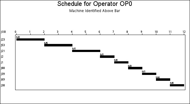
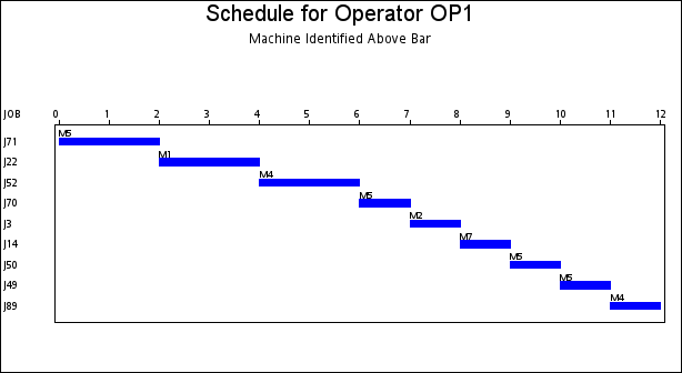
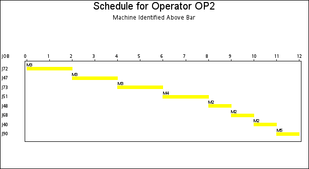
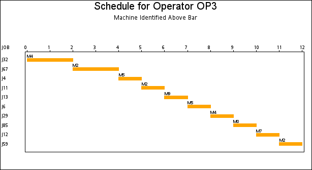
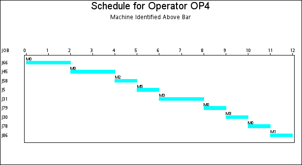
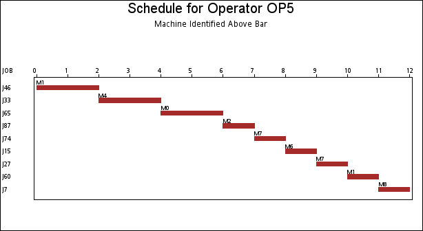
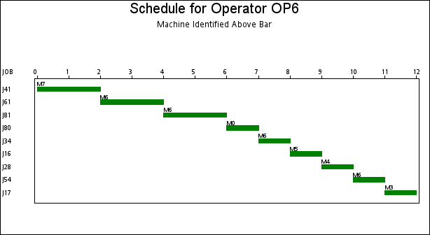
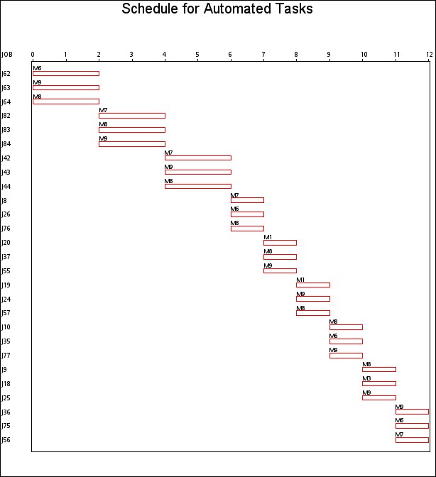
The resulting schedule is shown in a series of Gantt charts that are displayed in Output 1.2.1 and Output 1.2.2. In each of these Gantt charts, the vertical axis lists the different jobs, the horizontal bar represents the start and finish times for each of the jobs, and the text above each bar identifies the machine that the job is being processed on. Output 1.2.1 displays the schedule for the operator-assisted tasks—one for each operator. Output 1.2.2 shows the schedule for automated tasks—that is, those tasks not requiring operator intervention.
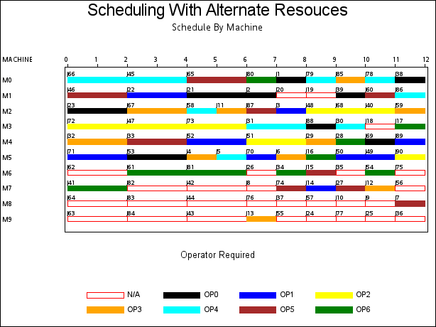
A more interesting Gantt chart is that of the resource schedule by machine, as shown in Output 1.2.3. This chart displays the schedule for each machine. Every row corresponds to a machine. Every bar on each row consists of multiple segments, and every segment represents a job that is processed on the machine. Each segment is also coded according to the operator assigned to it. The mapping of the coding is indicated in the legend. It is evident that the schedule is optimal since none of the machines or operators are idle at any time during the schedule.
Note: This procedure is experimental.
Copyright © 2008 by SAS Institute Inc., Cary, NC, USA. All rights reserved.