Time Series Analysis and Examples

Getting Started

Subsections:

Minimum AIC Model Selection
Nonstationary Data Analysis
Seasonal Adjustment
Miscellaneous Time Series Analysis Tools

Minimum AIC Model Selection

The time series model is automatically selected by using the AIC. The TSUNIMAR call estimates the univariate autoregressive model and computes the AIC. You need to specify the maximum lag or order of the AR process by using the MAXLAG= option or position the maximum lag as the sixth argument of the TSUNIMAR call.

Univariate AR Model

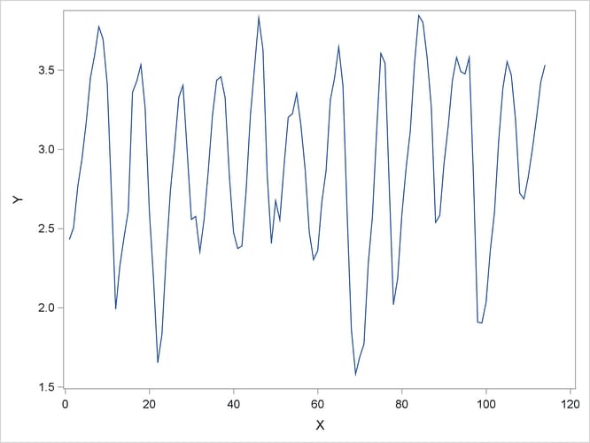
The following statements define and graph a time series, which is shown in Output 14.19:

proc iml;
y = { 2.430 2.506 2.767 2.940 3.169 3.450 3.594 3.774 3.695 3.411
      2.718 1.991 2.265 2.446 2.612 3.359 3.429 3.533 3.261 2.612
      2.179 1.653 1.832 2.328 2.737 3.014 3.328 3.404 2.981 2.557
      2.576 2.352 2.556 2.864 3.214 3.435 3.458 3.326 2.835 2.476
      2.373 2.389 2.742 3.210 3.520 3.828 3.628 2.837 2.406 2.675
      2.554 2.894 3.202 3.224 3.352 3.154 2.878 2.476 2.303 2.360
      2.671 2.867 3.310 3.449 3.646 3.400 2.590 1.863 1.581 1.690
      1.771 2.274 2.576 3.111 3.605 3.543 2.769 2.021 2.185 2.588
      2.880 3.115 3.540 3.845 3.800 3.579 3.264 2.538 2.582 2.907
      3.142 3.433 3.580 3.490 3.475 3.579 2.829 1.909 1.903 2.033
      2.360 2.601 3.054 3.386 3.553 3.468 3.187 2.723 2.686 2.821
      3.000 3.201 3.424 3.531 };
call series(1:ncol(y), y);

Output 14.19: Time Series Data

You can select the order of the AR process by finding the lag that minimizes the AIC. The following statements fit the various AR models. Notice that the first 20 observations are used as presample values. Output 14.20 shows that a model with a lag of 11 is the model that minimizes the AIC. The minimum AIC value is approximately $-298.1$ . The innovation variance of that model is 0.03. Output 14.21 shows the parameter estimates for the model.

call tsunimar(arcoef,ev,nar,aic) data=y opt={-1 1} maxlag=20;
print nar aic ev, arcoef;

Output 14.20: Time Series Statistics

nar	aic	ev
11	-298.1301	0.0331856

Output 14.21: Parameter Estimates

arcoef
1.181322
-0.551571
0.2313716
-0.17804
0.019874
-0.062573
0.0285691
-0.05071
0.1998957
0.1618192
-0.339086

Alternatively, you can invoke the TSUNIMAR subroutine as follows:

call tsunimar(arcoef,ev,nar,aic,y,20,{-1 1});

The optional arguments can be omitted. In this example, the argument MISSING is omitted, and thus the default value (MISSING=0) is used.

You can estimate the AR(11) model directly by specifying OPT= $\{ -1~ 0\}$ and using the first 11 observations as presample values. The AR(11) estimates that are shown in Output 14.22 are different from the minimum AIC estimates in Output 14.21 because the samples are slightly different. The following statements estimate and print the AR(11) estimates:

call tsunimar(arcoef11,ev,nar,aic,y,11,{-1 0});
print arcoef11;

Output 14.22: Parameter Estimates for AR(11) Model

arcoef11
1.1494157
-0.533719
0.2763117
-0.32642
0.1693359
-0.164108
0.0731226
-0.030428
0.151227
0.1928076
-0.3402

Multivariate VAR Model

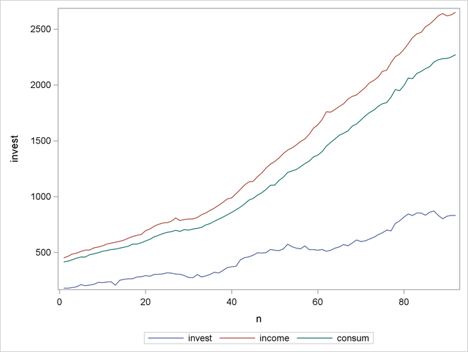
The minimum AIC procedure can also be applied to the vector autoregressive (VAR) model by using the TSMULMAR subroutine. The following DATA step defines a time series in three variables: investment, durable consumption, and consumption expenditures. The data are found in the appendix to Lütkepohl (1993). The series is plotted in Output 14.23.

data var3;
   input invest income consum @@;
   n = _N_;
datalines;
 180 451  415  179 465  421   185 485  434   192 493  448
 211 509  459  202 520  458   207 521  479   214 540  487
 231 548  497  229 558  510   234 574  516   237 583  525
 206 591  529  250 599  538   259 610  546   263 627  555
 264 642  574  280 653  574   282 660  586   292 694  602
 286 709  617  302 734  639   304 751  653   307 763  668
 317 766  679  314 779  686   306 808  697   304 785  688
 292 794  704  275 799  699   273 799  709   301 812  715
 280 837  724  289 853  746   303 876  758   322 897  779
 315 922  798  339 949  816   364 979  837   371 988  858
 375 1025 881  432 1063 905   453 1104 934   460 1131 968
 475 1137 983  496 1178 1013  494 1211 1034  498 1256 1064
 526 1290 1101 519 1314 1102  516 1346 1145  531 1385 1173
 573 1416 1216 551 1436 1229  538 1462 1242  532 1493 1267
 558 1516 1295 524 1557 1317  525 1613 1355  519 1642 1371
 526 1690 1402 510 1759 1452  519 1756 1485  538 1780 1516
 549 1807 1549 570 1831 1567  559 1873 1588  584 1897 1631
 611 1910 1650 597 1943 1685  603 1976 1722  619 2018 1752
 635 2040 1774 658 2070 1807  675 2121 1831  700 2132 1842
 692 2199 1890 759 2253 1958  782 2276 1948  816 2318 1994
 844 2369 2061 830 2423 2056  853 2457 2102  852 2470 2121
 833 2521 2145 860 2545 2164  870 2580 2206  830 2620 2225
 801 2639 2235 824 2618 2237  831 2628 2250  830 2651 2271
;

proc sgplot data=var3;
   series x=n y=invest;
   series x=n y=income;
   series x=n y=consum;
run;

Output 14.23: Multivariate Time Series Data

The following statements model the three variables as described in the section Multivariate Time Series Analysis. The maximum lag is specified as 10.

proc iml;
use var3;
read all var{invest income consum} into y;
close var3;
mdel = 1;  maice = 2;  misw = 0;
opt    = mdel || maice || misw;
maxlag = 10;  miss = 0;  print = 1;
call tsmulmar(ar_coef,variance,nar,aic,y,maxlag,opt,miss,print);
print nar aic;

Output 14.24: Statistics for Multivariate Series

nar	aic
3	1305.2256

Output 14.24 shows that the VAR(3) model minimizes the AIC and is selected as an appropriate model. However, the LISTING output from the AICs of the VAR(4) and VAR(5) models (not shown) indicates little difference from VAR(3). You can also choose VAR(4) or VAR(5) as an appropriate model in the context of minimum AIC because this AIC difference is much less than 1.

The TSMULMAR subroutine estimates the instantaneous response model with diagonal error variance. For more information about the instantaneous response model, see the section Multivariate Time Series Analysis. Therefore, it is possible to select the minimum AIC model independently for each equation. The best model is selected by specifying MAXLAG=5, as shown in the following statements:

call tsmulmar(arcoef,variance,nar,aic) data=y maxlag=5
   opt={1 1 0} print=1;
print variance, arcoef[c={"invest" "income" "consum"}];

Output 14.25: Model Selection via Instantaneous Response Model: Variance

variance
256.64375	29.803549	76.846777
29.803549	228.97341	119.60387
76.846777	119.60387	134.21764

Output 14.26: Model Selection via Instantaneous Response Model: Estimates

arcoef
invest	income	consum
13.312109	1.5459098	15.963897
0.8257397	0.2514803	0
0.0958916	1.0057088	0
0.0320985	0.3544346	0.4698934
0.044719	-0.201035	0
0.0051931	-0.023346	0
0.1169858	-0.060196	0.0483318
0.1867829	0	0
0.0216907	0	0
-0.117786	0	0.3500366
0.1541108	0	0
0.0178966	0	0
0.0461454	0	-0.191437
-0.389644	0	0
-0.045249	0	0
-0.116671	0	0

The error variance matrix is shown in Output 14.25. The AR coefficient matrix is shown in Output 14.26. You can print the intermediate results of the minimum AIC procedure by using the PRINT=2 option.

Notice that the AIC value depends on the MAXLAG=lag option and the number of parameters that are estimated. The minimum AIC VAR estimation procedure (MAICE=2) uses the following AIC formula:

$(T-\mi{lag}) \log (|\hat{\Sigma }|) + 2(p n^2 + n \delta )$

In this formula, p is the order of the n-variate VAR process, and $\delta = 1$ if the intercept is specified; otherwise, $\delta = 0$ . When you specify MAICE=1 or MAICE=0, the AIC is computed as the sum of AIC for each response equation. Consequently, there is an AIC difference of $n(n-1)$ , because the instantaneous response model contains the additional $n(n-1)/2$ response variables as regressors.

The following statements estimate the instantaneous response model. The results are shown in Output 14.27.

call tsmulmar(arcoef,ev,nar,aic) data=y maxlag=3 opt={1 0 0};
print nar aic, arcoef[c={"invest" "income" "consum"}];

Output 14.27: AIC from Instantaneous Response Model

nar	aic
3	1403.0762

arcoef
invest	income	consum
4.8245814	5.3559216	17.066894
0.8855926	0.3401741	-0.014398
0.1684523	1.0502619	0.107064
0.0891034	0.4591573	0.4473672
-0.059195	-0.298777	0.1629818
0.1128625	-0.044039	-0.088186
0.1684932	-0.025847	-0.025671
0.0637227	-0.196504	0.0695746
-0.226559	0.0532467	-0.099808
-0.303697	-0.139022	0.2576405

The following statements estimate the VAR model. The results are shown in Output 14.28.

call tsmulmar(arcoef,ev,nar,aic) data=y maxlag=3
     opt={1 2 0};
print nar aic, arcoef[c={"invest" "income" "consum"}];

Output 14.28: AIC from VAR Model

nar	aic
3	1397.0762

arcoef
invest	income	consum
4.8245814	5.3559216	17.066894
0.8855926	0.3401741	-0.014398
0.1684523	1.0502619	0.107064
0.0891034	0.4591573	0.4473672
-0.059195	-0.298777	0.1629818
0.1128625	-0.044039	-0.088186
0.1684932	-0.025847	-0.025671
0.0637227	-0.196504	0.0695746
-0.226559	0.0532467	-0.099808
-0.303697	-0.139022	0.2576405

The AIC that is computed from the instantaneous response model is greater than that obtained from the VAR model estimation by 6. Output 14.28 differs from Output 14.24 because different observations are used for estimation.

Nonstationary Data Analysis

The following examples show how to manage nonstationary data by using TIMSAC calls. In practice, time series are considered to be stationary when the expected values of first and second moments of the series do not change over time. This weak or covariance stationarity can be modeled by using the TSMLOCAR, TSMLOMAR, TSDECOMP, and TSTVCAR subroutines.

Univariate Stationary Data Analysis

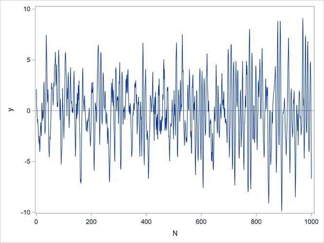
Output 14.29 shows the time series to be analyzed. The series consists of 1,000 observations.

data nonsta;
   input y @@;
   N = _N_;
datalines;
  .21232e1   .47451    -.171e-2  -.84434    -.10876e1
 -.84429    -.15320e1  -.21097e1 -.28282e1 -.30424e1

   ... more lines ...   

;

proc sgplot data=nonsta;
   refline 0 / axis=y;
   series x=N y=y;
run;

Output 14.29: Time Series Data

The following statements estimate the locally stationary model. The whole series (1,000 observations) is divided into three blocks of size 300 and one block of size 90, and the minimum AIC procedure is applied to each block of the data set. See the section Nonstationary Time Series for more details.

proc iml;
use nonsta;   read all var{y};   close nonsta;

mdel = -1;
lspan = 300; /* local span of data */
maice = 1;
opt = mdel || lspan || maice;
call tsmlocar(arcoef,ev,nar,aic,first,last)
                data=y maxlag=10 opt=opt print=2;

Estimation results are displayed with the graphs of power spectrum $(\log _{10}(f_{YY}(g)))$ , where $f_{YY}(g)$ is a rational spectral density function. See the section Spectral Analysis. The estimates for the first block and third block are shown in Output 14.30 and Output 14.33, respectively. Because the first block and the second block do not have any sizable difference, the pooled model (AIC=45.892) is selected instead of the moving model (AIC=46.957) in Output 14.31. However, you can notice a slight change in the shape of the spectrum of the third block of the data (observations 611 through 910). See Output 14.32 and Output 14.34 for comparison. The moving model is selected since the AIC (106.830) of the moving model is smaller than that of the pooled model (108.867).

Output 14.30: Locally Stationary Model for First Block

SAS Output

line
INITIAL LOCAL MODEL: N_CURR = 300
NAR_CURR = 8 AIC = 37.583203



..........................CURRENT MODEL.........................
. .
. .
. .
. M AR Coefficients: AR(M) .
. .
. 1 1.605717 .
. 2 -1.245350 .
. 3 1.014847 .
. 4 -0.931554 .
. 5 0.394230 .
. 6 -0.004344 .
. 7 0.111608 .
. 8 -0.124992 .
. .
. .
. AIC = 37.5832030 .
. Innovation Variance = 1.067455 .
. .
. .
. INPUT DATA START = 11 FINISH = 310 .
................................................................

Output 14.31: Locally Stationary Model Comparison

SAS Output

line
--- THE FOLLOWING TWO MODELS ARE COMPARED ---

MOVING MODEL: (N_PREV = 300, N_CURR = 300)
NAR_CURR = 7 AIC = 46.957398
CONSTANT MODEL: N_POOLED = 600
NAR_POOLED = 8 AIC = 45.892350

*** CONSTANT MODEL ADOPTED ***



..........................CURRENT MODEL.........................
. .
. .
. .
. M AR Coefficients: AR(M) .
. .
. 1 1.593890 .
. 2 -1.262379 .
. 3 1.013733 .
. 4 -0.926052 .
. 5 0.314480 .
. 6 0.193973 .
. 7 -0.058043 .
. 8 -0.078508 .
. .
. .
. AIC = 45.8923501 .
. Innovation Variance = 1.047585 .
. .
. .
. INPUT DATA START = 11 FINISH = 610 .
................................................................

Output 14.32: Power Spectrum for First and Second Blocks

SAS Output

line
POWER SPECTRAL DENSITY
20.00+
\|
\|
\|
\|
\| XXXX
XXX XX XXX
\| XXXX
\| X
\|
10.00+
\| X
\|
\| X
\|
\| X XX
\| X
\| X X
\|
\| X X X
0+ X
\| X X X
\| XX XX
\| XXXX X
\|
\| X
\| X
\|
\| X
\| X
-10.0+ X
\| XX
\| XX
\| XX
\| XXX
\| XXXXXX
\|
\|
\|
\|
-20.0+-----------+-----------+-----------+-----------+-----------+
0.0 0.1 0.2 0.3 0.4 0.5

FREQUENCY

Output 14.33: Locally Stationary Model for Third Block

SAS Output

line
--- THE FOLLOWING TWO MODELS ARE COMPARED ---

MOVING MODEL: (N_PREV = 600, N_CURR = 300)
NAR_CURR = 7 AIC = 106.829869
CONSTANT MODEL: N_POOLED = 900
NAR_POOLED = 8 AIC = 108.867091

*************************************
*** ***
*** NEW MODEL ADOPTED ***
*** ***
*************************************



..........................CURRENT MODEL.........................
. .
. .
. .
. M AR Coefficients: AR(M) .
. .
. 1 1.648544 .
. 2 -1.201812 .
. 3 0.674933 .
. 4 -0.567576 .
. 5 -0.018924 .
. 6 0.516627 .
. 7 -0.283410 .
. .
. .
. AIC = 60.9375188 .
. Innovation Variance = 1.161592 .
. .
. .
. INPUT DATA START = 611 FINISH = 910 .
................................................................

Output 14.34: Power Spectrum for Third Block

SAS Output

line
POWER SPECTRAL DENSITY
20.00+ X
\| X
\| X
\| X
\| XXX
\| XXXXX
\| XX
XX X
\|
\|
10.00+ X
\|
\|
\| X
\|
\| X
\| X
\| X X
\| X
\| X X
0+ X X X
\| X
\| X XX X
\| XXXXXX
\| X
\|
\| X
\|
\| X
\| X
-10.0+ X
\| XX
\| XX XXXXX
\| XXXXXXX
\|
\|
\|
\|
\|
\|
-20.0+-----------+-----------+-----------+-----------+-----------+
0.0 0.1 0.2 0.3 0.4 0.5

FREQUENCY

The moving model is selected because there is a structural change in the last block of data. (The FIRST and LAST variables contain the values 911 amd 1,000, respectively; this correspond to observations 911 through 1,000.) The final estimates are stored in variables ARCOEF, EV, NAR, AIC, FIRST, and LAST. The final estimates and spectrum are given in Output 14.35 and Output 14.36, respectively. The power spectrum of the final model (Output 14.36) is significantly different from that of the first and second blocks (see Output 14.32).

Output 14.35: Locally Stationary Model for Last Block

SAS Output

line
--- THE FOLLOWING TWO MODELS ARE COMPARED ---

MOVING MODEL: (N_PREV = 300, N_CURR = 90)
NAR_CURR = 6 AIC = 139.579012
CONSTANT MODEL: N_POOLED = 390
NAR_POOLED = 9 AIC = 167.783711

*************************************
*** ***
*** NEW MODEL ADOPTED ***
*** ***
*************************************



..........................CURRENT MODEL.........................
. .
. .
. .
. M AR Coefficients: AR(M) .
. .
. 1 1.181022 .
. 2 -0.321178 .
. 3 -0.113001 .
. 4 -0.137846 .
. 5 -0.141799 .
. 6 0.260728 .
. .
. .
. AIC = 78.6414932 .
. Innovation Variance = 2.050818 .
. .
. .
. INPUT DATA START = 911 FINISH = 1000 .
................................................................

Output 14.36: Power Spectrum for Last Block

SAS Output

line
POWER SPECTRAL DENSITY
30.00+
\|
\|
\|
\|
\| X
\|
\| X
\|
\|
20.00+ X
\|
\|
\| X X
\|
\| X
XXX X
\| XXXXX X
\|
\|
10.00+ X
\|
\| X
\|
\| X
\|
\| X
\| X
\| X
\| XX
0+ XX XXXXXX
\| XXXXXX XX
\| XX
\| XX XX
\| XX XXXX
\| XXXXXXXXX
\|
\|
\|
\|
-10.0+-----------+-----------+-----------+-----------+-----------+
0.0 0.1 0.2 0.3 0.4 0.5

FREQUENCY

Multivariate Stationary Data Analysis

The multivariate analysis for locally stationary data is a straightforward extension of the univariate analysis. This section uses data related to the rudder setting and yaw of an aircraft. A plot of the data is shown in Output 14.37.

data Aircraft;
input Rudder Yawing @@;
Time = _N_;
datalines;
515 -96 553 -56 544 -57 512 -61 583   8 

   ... more lines ...   

;

proc sgplot data=Aircraft;
   refline 0 / axis=y;
   series x=Time y=Rudder;
   series x=Time y=Yawing;
   yaxis label="Y";
run;

Output 14.37: Bivariate Time Series Data

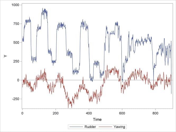
The following statements estimate bivariate locally stationary VAR models. The selected model is the VAR(7) process with some zero coefficients over the last block of data. There seems to be a structural difference between observations from 11 to 610 and those from 611 to 896.

proc iml;
use Aircraft;
read all var {rudder yawing} into y;
close Aircraft;

c = {0.01795 0.02419};
y = y # c;   /*-- calibration of data --*/
mdel = -1;
lspan = 300; /* local span of data */
maice = 1;
call tsmlomar(arcoef,ev,nar,aic,first,last) data=y maxlag=10
        opt = (mdel || lspan || maice) print=1;

The results of the analysis are shown in Output 14.38.

Output 14.38: Locally Stationary VAR Model Analysis

SAS Output

line
--- THE FOLLOWING TWO MODELS ARE COMPARED ---

MOVING MODEL: (N_PREV = 600, N_CURR = 286)
NAR_CURR = 7 AIC = -823.845234
CONSTANT MODEL: N_POOLED = 886
NAR_POOLED = 10 AIC = -716.818588

*************************************
*** ***
*** NEW MODEL ADOPTED ***
*** ***
*************************************



..........................CURRENT MODEL.........................
. .
. .
. .
. M AR Coefficients .
. .
. 1 0.932904 -0.130964 .
. -0.024401 0.599483 .
. 2 0.163141 0.266876 .
. -0.135605 0.377923 .
. 3 -0.322283 0.178194 .
. 0.188603 -0.081245 .
. 4 0.166094 -0.304755 .
. -0.084626 -0.180638 .
. 5 0 0 .
. 0 -0.036958 .
. 6 0 0 .
. 0 0.034578 .
. 7 0 0 .
. 0 0.268414 .
. .
. .
. AIC = -114.6911872 .
. .
. Innovation Variance .
. .
. 1.069929 0.145558 .
. 0.145558 0.563985 .
. .
. .
. INPUT DATA START = 611 FINISH = 896 .
................................................................

A Time Series Decomposition

Consider the time series decomposition

$y_ t = T_ t + S_ t + u_ t + \epsilon _ t$

where $T_ t$ and $S_ t$ are trend and seasonal components, respectively, and $u_ t$ is a stationary AR(p) process. The annual real GNP series in Example 14.1 is analyzed under second difference stochastic constraints on the trend component and the stationary AR(2) process.

$\begin{eqnarray*} T_ t & = & 2T_{t-1} - T_{t-2} + w_{1t} \\[0.05in] u_ t & = & \alpha _1 u_{t-1} + \alpha _2 u_{t-2} + w_{2t} \end{eqnarray*}$

The seasonal component is ignored if you specify SORDER=0. Therefore, the following state space model is estimated:

$\begin{eqnarray*} y_ t & = & \mb{H}\mb{z}_ t + \epsilon _ t \\[0.05in] \mb{z}_ t & = & \mb{F}\mb{z}_{t-1} + \mb{w}_ t \end{eqnarray*}$

where

$\begin{eqnarray*} \mb{H} & = & \left[ \begin{array}{cccc} 1 & 0 & 1 & 0 \end{array} \right] \\[0.05in] \mb{F} & = & \left[ \begin{array}{cccc} 2 & -1 & 0 & 0 \\ 1 & 0 & 0 & 0 \\ 0 & 0 & \alpha _1 & \alpha _2 \\ 0 & 0 & 1 & 0 \end{array} \right] \\[0.05in] \mb{z}_ t & = & (T_ t, T_{t-1}, u_ t, u_{t-1})^{\prime } \\[0.05in] \mb{w}_ t & = & (w_{1t}, 0, w_{2t}, 0)^{\prime } \sim \left(0, \left[ \begin{array}{cccc} \sigma _1^2 & 0 & 0 & 0 \\ 0 & 0 & 0 & 0 \\ 0 & 0 & \sigma _2^2 & 0 \\ 0 & 0 & 0 & 0 \end{array} \right] \right) \end{eqnarray*}$

The parameters of this state space model are $\sigma ^2_1$ , $\sigma ^2_2$ , $\alpha _1$ , and $\alpha _2$ . The following statements compute the decomposition:

proc iml;
use gnp;
read all var {y};
close gnp;
mdel  = 0;  trade = 0;  year  = 0;
period= 0;  log   = 0;  maxit = 100;
update = .; /* use default update method      */
line   = .; /* use default line search method */
sigmax = 0; /* no upper bound for variances   */
back = 100;
opt = mdel || trade || year || period || log || maxit ||
      update || line || sigmax || back;
call tsdecomp(cmp,coef,aic) data=y order=2 sorder=0 nar=2
     npred=5 opt=opt icmp={1 3} print=1;

The estimated parameters are printed when you specify the PRINT= option. In Output 14.39, the estimated variances are printed under the title of TAU2(I), showing that $\hat{\sigma }_1^2=2.915$ and $\hat{\sigma }_2^2=113.9577$ . The AR coefficient estimates are $\hat{\alpha }_1=1.397$ and $\hat{\alpha }_2=-0.595$ . These estimates are also stored in the output matrix COEF.

Output 14.39: Nonstationary Time Series and State Space Modeling

SAS Output

line

<<

--- PARAMETER VECTOR ---

1.607423E-01 6.283820E+00 8.761627E-01 -5.94879E-01

--- GRADIENT ---

3.352158E-04 5.237221E-06 2.907539E-04 -1.24376E-04


LIKELIHOOD = -249.937193 SIG2 = 18.135085
AIC = 509.874385

I TAU2(I) AR(I) PARCOR(I)
1 2.915075 1.397374 0.876163
2 113.957607 -0.594879 -0.594879

The trend and stationary AR components are estimated by using the smoothing method, and out-of-sample forecasts are computed by using a Kalman filter prediction algorithm. The trend and AR components are stored in the matrix CMP since the ICMP={1 3} option is specified. The last 10 observations of the original series Y and the last 15 observations of two components are shown in Output 14.40. Note that the first column of CMP is the trend component and the second column is the AR component. The last 5 observations of the CMP matrix are out-of-sample forecasts.

y = y[52:61];
cmp = cmp[52:66,];
obs = T(52:66);
print obs y cmp;

Output 14.40: Smoothed and Predicted Values of Two Components

obs	y	cmp
52	487.7	-41.37417
53	497.2	201.99968
54	529.8	-31.05757
55	551	209.65589
56	581.1	-17.65476
57	617.8	217.82432
58	658.1	-17.0613
59	675.2	226.44692
60	706.6	-30.21502
61	724.7	235.85739
62		-27.7061
63		245.85384
64		-17.31128
65		256.43509
66		6.1997939

Seasonal Adjustment

Consider the simple time series decomposition

$y_ t = T_ t + S_ t + \epsilon _ t$

The TSBAYSEA subroutine computes seasonally adjusted series by estimating the seasonal component. The seasonally adjusted series is computed as $y_ t^* = y_ t - \hat{S}_ t$ . The details of the adjustment procedure are given in the section Bayesian Seasonal Adjustment.

The monthly labor force series (1972–1978) are analyzed. You do not need to specify the options vector if you want to use the default options. However, you should change OPT[2] when the data frequency is not monthly (OPT[2]=12). The NPRED= option produces the multistep forecasts for the trend and seasonal components. The stochastic constraints are specified as ORDER=2 and SORDER=1.

$\begin{eqnarray*} T_ t & = & 2T_{t-1} - T_{t-2} + w_{1t} \\ S_ t & = & -S_{t-1} - \cdots - S_{t-11} + w_{2t} \end{eqnarray*}$

In Output 14.41, the first column shows the trend components; the second column shows the seasonal components; the third column shows the forecasts; the fourth column shows the seasonally adjusted series; the last column shows the value of ABIC. The last 12 rows are the forecasts. The output is generated by using the following statements:

   proc iml;
   y = { 5447 5412 5215 4697 4344 5426   
         5173 4857 4658 4470 4268 4116    
         4675 4845 4512 4174 3799 4847    
         4550 4208 4165 3763 4056 4058    
         5008 5140 4755 4301 4144 5380    
         5260 4885 5202 5044 5685 6106    
         8180 8309 8359 7820 7623 8569    
         8209 7696 7522 7244 7231 7195    
         8174 8033 7525 6890 6304 7655    
         7577 7322 7026 6833 7095 7022    
         7848 8109 7556 6568 6151 7453    
         6941 6757 6437 6221 6346 5880 }`; 

   call tsbaysea(trend,season,series,adj,abic)
        data=y order=2 sorder=1 npred=12 print=2;
   print trend season series adj abic;

Output 14.41: Trend and Seasonal Component Estimates and Forecasts

obs	trend	season	series	adj	abic
1	4843.2502	576.86675	5420.1169	4870.1332	874.04585
2	4848.6664	612.79607	5461.4624	4799.2039
3	4871.2876	324.02004	5195.3077	4890.98
4	4896.6633	-198.7601	4697.9032	4895.7601
5	4922.9458	-572.5562	4350.3896	4916.5562
.	.	.	.	.
71	6551.6017	-266.2162	6285.3855	6612.2162
72	6388.9012	-440.3472	5948.5539	6320.3472
73	6226.2006	650.7707	6876.9713
74	6063.5001	800.93733	6864.4374
75	5900.7995	396.19866	6296.9982
76	5738.099	-340.2852	5397.8137
77	5575.3984	-719.1146	4856.2838
78	5412.6979	553.19764	5965.8955
79	5249.9973	202.06582	5452.0631
80	5087.2968	-54.44768	5032.8491
81	4924.5962	-295.2747	4629.3215
82	4761.8957	-487.6621	4274.2336
83	4599.1951	-266.1917	4333.0034
84	4436.4946	-440.3354	3996.1591

The estimated spectral density function of the irregular series $\hat{\epsilon }_ t$ is shown in Output 14.42 and Output 14.43.

Output 14.42: Spectrum of Irregular Component

SAS Output

line
I Rational 0.0 10.0 20.0 30.0 40.0 50.0 60.0
Spectrum +---------+---------+---------+---------+---------+---------+
0 1.366798E+00 \|* ===>X
1 1.571261E+00 \|*
2 2.414836E+00 \| *
3 5.151906E+00 \| *
4 1.634887E+01 \| *
5 8.085674E+01 \| *
6 3.805530E+02 \| *
7 8.082536E+02 \| *
8 6.366350E+02 \| *
9 3.479435E+02 \| *
10 3.872650E+02 \| * ===>X
11 1.264805E+03 \| *
12 1.726138E+04 \| *
13 1.559041E+03 \| *
14 1.276516E+03 \| *
15 3.861089E+03 \| *
16 9.593184E+03 \| *
17 3.662145E+03 \| *
18 5.499783E+03 \| *
19 4.443303E+03 \| *
20 1.238135E+03 \| * ===>X
21 8.392131E+02 \| *
22 1.258933E+03 \| *
23 2.932003E+03 \| *
24 1.857923E+03 \| *
25 1.171437E+03 \| *
26 1.611958E+03 \| *
27 4.822498E+03 \| *
28 4.464961E+03 \| *
29 1.951547E+03 \| *
30 1.653182E+03 \| * ===>X
31 2.308152E+03 \| *
32 5.475758E+03 \| *
33 2.349584E+04 \| *
34 5.266969E+03 \| *
35 2.058667E+03 \| *
36 2.215595E+03 \| *
37 8.181540E+03 \| *
38 3.077329E+03 \| *
39 7.577961E+02 \| *
40 5.057636E+02 \| * ===>X
41 7.312090E+02 \| *
42 3.131377E+03 \| * ===>T
43 8.173276E+03 \| *
44 1.958359E+03 \| *
45 2.216458E+03 \| *
46 4.215465E+03 \| *
47 9.659340E+02 \| *
48 3.758466E+02 \| *
49 2.849326E+02 \| *
50 3.617848E+02 \| * ===>X
51 7.659839E+02 \| *
52 3.191969E+03 \| *

Output 14.43: continued

SAS Output

line
53 1.768107E+04 \| *
54 5.281385E+03 \| *
55 2.959704E+03 \| *
56 3.783522E+03 \| *
57 1.896625E+04 \| *
58 1.041753E+04 \| *
59 2.038940E+03 \| *
60 1.347568E+03 \| * ===>X

X: If peaks (troughs) appear
at these frequencies,
try lower (higher) values
of rigid and watch ABIC
T: If a peaks appears here
try trading-day adjustment

Miscellaneous Time Series Analysis Tools

The TSPRED Subroutine

The forecast values of multivariate time series are computed by using the TSPRED call. In the following example, the multistep-ahead forecasts are produced from the VARMA(2,1) estimates. Because the VARMA model is estimated by using the mean deleted series, you should specify the CONSTANT = –1 option. You need to provide the original series instead of the mean deleted series to get the correct predictions. The forecast variance MSE and the impulse response function IMPULSE are also produced.

The VARMA( $p,q$ ) model is written

$\mb{y}_ t + \sum _{i=1}^ p \mb{A}_ i\mb{y}_{t-i} = \epsilon _ t + \sum _{i=1}^ q \mb{M}_ i\epsilon _{t-i}$

Then the COEF matrix is constructed by stacking matrices $\bA _1,\ldots ,\bA _ p,$ $\bM _1,\ldots ,\bM _ q$ . The following statements analyze the data, which contains 40 observations and four variables:

proc iml;
c = { 264 235 239 239 275 277 274 334 334 306
      308 309 295 271 277 221 223 227 215 223
      241 250 270 303 311 307 322 335 335 334
      309 262 228 191 188 215 215 249 291 296 };
f = { 690 690 688 690 694 702 702 702 700 702
      702 694 708 702 702 708 700 700 702 694
      698 694 700 702 700 702 708 708 710 704
      704 700 700 694 702 694 710 710 710 708 };
t = { 1152 1288 1288 1288 1368 1456 1656 1496 1744 1464
      1560 1376 1336 1336 1296 1296 1280 1264 1280 1272
      1344 1328 1352 1480 1472 1600 1512 1456 1368 1280
      1224 1112 1112 1048 1176 1064 1168 1280 1336 1248 };
p = { 254.14 253.12 251.85 250.41 249.09 249.19 249.52 250.19
      248.74 248.41 249.95 250.64 250.87 250.94 250.96 251.33
      251.18 251.05 251.00 250.99 250.79 250.44 250.12 250.19
      249.77 250.27 250.74 250.90 252.21 253.68 254.47 254.80
      254.92 254.96 254.96 254.96 254.96 254.54 253.21 252.08 };

y = c` || f` || t` || p`;
/* AR coefficients */
ar = {  .82028   -.97167    .079386   -5.4382,
       -.39983    .94448    .027938   -1.7477,
       -.42278  -2.3314    1.4682    -70.996,
        .031038  -.019231  -.0004904   1.3677,
       -.029811   .89262   -.047579    4.7873,
        .31476    .0061959 -.012221    1.4921,
        .3813    2.7182    -.52993    67.711,
       -.020818   .01764    .00037981  -.38154 };
/* AR coefficients */
ma = {  .083035 -1.0509     .055898   -3.9778,
       -.40452    .36876    .026369    -.81146,
        .062379 -2.6506     .80784   -76.952,
        .03273   -.031555  -.00019776  -.025205 };
coef = ar // ma;          /* stack the coefficients */
ev = { 188.55   6.8082    42.385   .042942,
       6.8082   32.169    37.995  -.062341,
       42.385   37.995    5138.8  -.10757,
       .042942  -.062341  -.10757  .34313 };

nar = 2; nma = 1;
call tspred(forecast,impulse,mse,y,coef,nar,nma,ev,
               5,nrow(y),-1);

If you write the data and the predicted values to a SAS data set, you can use the SGPANEL procedure to visualize the original series and the forecasts. The result is shown in Output 14.44.

Output 14.44: Multivariate ARMA Prediction

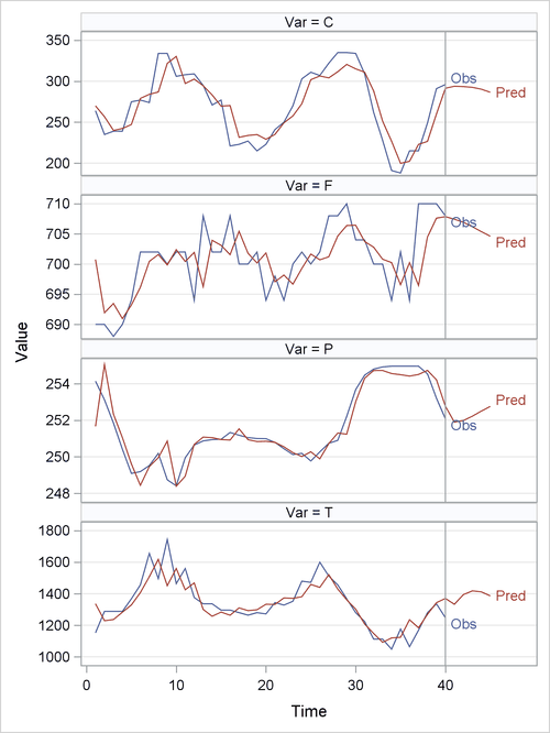
The forecast variable contains 45 observations. The first 40 rows are one-step predictions. The last five rows contain the five-step forecast values of the variables C, F, T, and P. You can construct the confidence interval for these forecasts by using the mean square error matrix, MSE. See the section Multivariate Time Series Analysis for more details about impulse response functions and the mean square error matrix.

The TSROOT Subroutine

The TSROOT call computes the polynomial roots of the AR and MA equations. When the AR(p) process is written

$y_ t = \sum _{i=1}^ p \alpha _ i y_{t-i} + \epsilon _ t$

you can specify the following polynomial equation:

$z^ p - \sum _{i=1}^ p \alpha _ i z^{p-i} = 0$

When all p roots of the preceding equation are inside the unit circle, the AR(p) process is stationary. The MA(q) process is invertible if the following polynomial equation has all roots inside the unit circle:

$z^ q + \sum _{i=1}^ q \theta _ i z^{q-i} = 0$

where $\theta _ i$ are the MA coefficients.

For example, the following program analyzes the time series data that are shown in Output 14.19. The TSUNIMAR subroutine (see Output 14.45) selects the best AR model and estimates the AR coefficients, as shown in Output 14.45.

proc iml;
y = { 2.430 2.506 2.767 2.940 3.169 3.450 3.594 3.774 3.695 3.411
      2.718 1.991 2.265 2.446 2.612 3.359 3.429 3.533 3.261 2.612
      2.179 1.653 1.832 2.328 2.737 3.014 3.328 3.404 2.981 2.557
      2.576 2.352 2.556 2.864 3.214 3.435 3.458 3.326 2.835 2.476
      2.373 2.389 2.742 3.210 3.520 3.828 3.628 2.837 2.406 2.675
      2.554 2.894 3.202 3.224 3.352 3.154 2.878 2.476 2.303 2.360
      2.671 2.867 3.310 3.449 3.646 3.400 2.590 1.863 1.581 1.690
      1.771 2.274 2.576 3.111 3.605 3.543 2.769 2.021 2.185 2.588
      2.880 3.115 3.540 3.845 3.800 3.579 3.264 2.538 2.582 2.907
      3.142 3.433 3.580 3.490 3.475 3.579 2.829 1.909 1.903 2.033
      2.360 2.601 3.054 3.386 3.553 3.468 3.187 2.723 2.686 2.821
      3.000 3.201 3.424 3.531 };

call tsunimar(ar,innov_var,nar,aic) data=y maxlag=5
     opt=({-1 1}) print=0;
lag = (1:5)`;
print lag ar, aic innov_var;

Output 14.45: Minimum AIC AR Estimation

lag	ar
1	1.3003068
2	-0.72328
3	0.2421928
4	-0.378757
5	0.1377273

aic	innov_var
-318.6138	0.0490554

You can obtain the associated roots by calling the TSROOT subroutine. The TSROOT subroutine expects to receive complex AR or MA coefficients, whereas the matrix from the TSUNIMAR subroutine contains real coefficients. To represent complex coefficients, append a column of zeros (the value of the imaginary coefficients) and pass in the two-column matrix to the TSROOT subroutine by using the MATIN= argument, as follows:

/*-- set up complex coefficient matrix --*/
ar_cx = ar || j(nrow(ar),1,0);
call tsroot(root) matin=ar_cx nar=nar nma=0;

The output of the TSROOT subroutine is the ROOT matrix, which has two columns and five rows. Each row contains the real and imaginary parts of the roots of the characteristic polynomial $z^5 -\alpha _1 z^4 - \alpha _2 z^3 - \alpha _3 z^2 - \alpha _4 z^1 - \alpha _5$ , where the $\alpha _ i$ are the AR coefficients. Sometimes it is useful to display other information about the roots, as shown in Output 14.9 and Output 14.13. The following module prints the roots, their moduli, and their angles in the complex plane.

start PrintRootInfo(z); /* print Re(z), Im(z), |z|), and Arg(z) */
   m = j(nrow(z), 6);
   m[,1] = t(1:nrow(z));
   m[,{2 3}] = z;
   m[,4] = sqrt(z[,##]);        /* modulus */
   m[,5] = atan2(z[,2], z[,1]); /* atan(I/R) */
   m[,6] = m[,5] * 180 / constant('pi'); /* degree */
   print m[L="Roots of AR Characteristic Polynomial"
           c={I "Real" "Imaginary" "MOD(z)" "ATan(I/R)" "Deg"}];
finish;
run PrintRootInfo(root);

The result is shown in Output 14.46. All roots are within the unit circle. The modulus values of the fourth and fifth roots are sizable (0.9194).

Output 14.46: Roots of AR Characteristic Polynomial Equation

Roots of AR Characteristic Polynomial
	I	Real	Imaginary	MOD(z)	ATan(I/R)	Deg
ROW1	1	-0.297546	0.5599112	0.6340618	2.0592605	117.98694
ROW2	2	-0.297546	-0.559911	0.6340618	-2.059261	-117.9869
ROW3	3	0.4052936	0	0.4052936	0	0
ROW4	4	0.7450529	0.5386556	0.9193768	0.6259805	35.866038
ROW5	5	0.7450529	-0.538656	0.9193768	-0.62598	-35.86604

The TSROOT subroutine can also recover the polynomial coefficients if the roots are provided as an input. Specify the QCOEF=1 option when you want to compute the polynomial coefficients instead of polynomial roots. The results are shown in Output 14.47, which you should compare with Output 14.45.

call tsroot(ar_cx) matin=root nar=nar qcoef=1 nma=0;
reset fuzz;
print (lag || ar_cx)[L="Polyomial Coefficients"
                     c={"I" "AR(real)" "AR(imag)"}];

Output 14.47: Polynomial Coefficients

Polyomial Coefficients
I	AR(real)	AR(imag)
1	1.3003068	0
2	-0.72328	0
3	0.2421928	0
4	-0.378757	0
5	0.1377273	0