Time Series Analysis and Examples

Getting Started

Subsections:

Stationary VAR Process
Nonstationary VAR Process

Stationary VAR Process

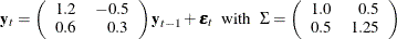
The following equation describes a first-order stationary vector autoregressive model with zero mean:

$\begin{eqnarray*} \mb{y}_{t} = \left( \begin{array}{rr} 1.2 & -0.5 \\ 0.6 & 0.3 \\ \end{array} \right) \mb{y}_{t-1} + {\bepsilon }_ t ~ ~ \textrm{with}~ ~ \Sigma = \left( \begin{array}{rr} 1.0 & 0.5 \\ 0.5 & 1.25 \\ \end{array} \right) \end{eqnarray*}$

The following statements simulate 100 observations for the model:

proc iml;
/* stationary VAR(1) model */
sig = {1.0  0.5, 0.5 1.25};
phi = {1.2 -0.5, 0.6 0.3};
call varmasim(yt,phi) sigma=sig n=100 seed=3243;

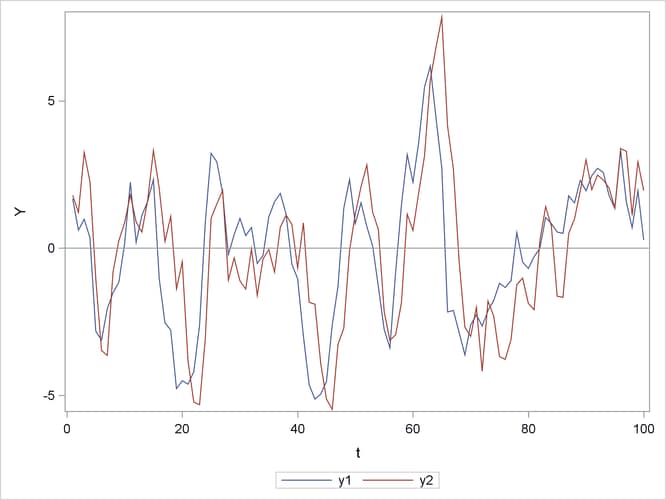
The stationary VAR(1) process is shown in Output 14.8.

Output 14.8: Plot of Generated VAR(1) Process (VARMASIM)

The following statements compute the roots of the characteristic function:

call vtsroot(root,phi);
print root[c={R I 'Mod' 'ATan' 'Deg'}];

Output 14.9: Roots of VAR(1) Model (VTSROOT)

root
R	I	Mod	ATan	Deg
0.75	0.3122499	0.8124038	0.3945069	22.603583
0.75	-0.31225	0.8124038	-0.394507	-22.60358

In Output 14.9, the first column displays the real part (R) of the root of the characteristic function, and the second column shows the imaginary part (I). The third column displays the modulus, the square root of $R^2+I^2$ . The fourth column shows the $\tan ^{-1}(I/R)$ , measured in radians, and the last column shows the same measurement in degrees. The third column shows that the moduli are less than 1, so the series is stationary.

The following statements compute five lags of cross-covariance matrices:

call varmacov(crosscov,phi) sigma=sig lag=5;
lag = {'0','','1','','2','','3','','4','','5',''};
print lag crosscov;

Output 14.10: Cross-Covariance Matrices of VAR(1) Model (VARMACOV)

lag	crosscov
0	5.3934173	3.8597124
	3.8597124	5.0342051
1	4.5422445	4.3939641
	2.1145523	3.826089
2	3.2537114	4.0435359
	0.6244183	2.4165581
3	1.8826857	3.1652876
	-0.458977	1.0996184
4	0.676579	2.0791977
	-1.100582	0.0544993
5	-0.227704	1.0297067
	-1.347948	-0.643999

In each matrix in Output 14.10, the diagonal elements correspond to the autocovariance functions of each time series. The off-diagonal elements correspond to the cross-covariance functions between the two series.

The following statements evaluate the log-likelihood function of the VAR(1) model:

call varmalik(lnl,yt,phi) sigma=sig;
labl = {"LogLik", "SumLogDet", "SSE"};
print lnl[rowname=labl];

Output 14.11: Log-Likelihood Function of VAR(1) Model (VARMALIK)

lnl
LogLik	-113.4708
SumLogDet	2.5058678
SSE	224.43567

In Output 14.11, the first row displays the value of log-likelihood function; the second row shows the sum of the log determinant of the innovation variance; the last row displays the weighted sum of squares of residuals.

Nonstationary VAR Process

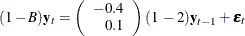
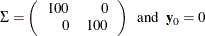
The following equation describes an error-correction model with a cointegrated rank of 1:

$\begin{eqnarray*} (1-B) \mb{y}_{t} = \left( \begin{array}{r} -0.4 \\ 0.1 \\ \end{array} \right) ( 1\; -2 ) \mb{y}_{t-1} + {\bepsilon }_ t \end{eqnarray*}$

with

$\begin{eqnarray*} \Sigma = \left( \begin{array}{rr} 100 & 0 \\ 0 & 100 \\ \end{array} \right) ~ ~ \textrm{and}~ ~ \mb{y}_0 = 0 \end{eqnarray*}$

In the equation, $\mb{y}_{t}$ is a $2\times 1$ vector. On the right hand side of the equation, the $1\times 2$ row vector $( 1\; -2 )$ multiplies the vector $\mb{y}_{t-1}$ to form a scalar linear combination of components.

The following statements generate simulated data:

proc iml;
/* nonstationary  model */
sig = 100*i(2);
phi = {0.6 0.8, 0.1 0.8};   /* derived model */
call varmasim(yt,phi) sigma=sig n=100 seed=1324;

Output 14.12: Plot of Generated Nonstationary Vector Process (VARMASIM)

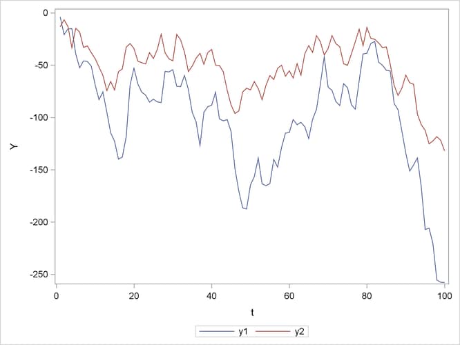
The nonstationary correlated processes are shown in Output 14.12.

The following statements compute the roots of the characteristic function:

call vtsroot(root,phi);
print root[c={R I 'Mod' 'ATan' 'Deg'}];

Output 14.13: Roots of Nonstationary VAR(1) Model (VTSROOT)

root
R	I	Mod	ATan	Deg
1	0	1	0	0
0.4	0	0.4	0	0

In Output 14.13, the first column displays the real part (R) of the root of the characteristic function, and the second column displays the imaginary part (I). The third column shows that a modulus is greater than or equal to 1, so the series is nonstationary.