Wavelet Analysis

Wavelet scalograms communicate the time frequency localization property of the discrete wavelet transform. In this plot each detail coefficient is plotted as a filled rectangle whose color corresponds to the magnitude of the coefficient. The location and size of the rectangle are related to the time interval and the frequency range for this coefficient. Coefficients at low levels are plotted as wide and short rectangles to indicate that they localize a wide time interval but a narrow range of frequencies in the data. In contrast, rectangles for coefficients at high levels are plotted thin and tall to indicate that they localize small time ranges but large frequency ranges in the data. The heights of the rectangles grow as a power of 2 as the level increases. If you include all levels of coefficients in such a plot, the heights of the rectangles at the lowest levels are so small that they are not visible. You can use an option to plot the heights of the rectangles on a logarithmic scale. This results in rectangles of uniform height but requires that you interpret the frequency localization of the coefficients with care.
The following statement produces a scalogram plot of all levels with "SureShrink" thresholding applied:
      call scalogram(decomp,&SureShrink, , ,0.25,
                     'log',"Quartz Spectrum");
The sixth argument specifies that the rectangle heights are to be plotted on a logarithmic scale. The role of the fifth argument
(0.25) is to amplify the magnitude of the small detail coefficients. This is necessary since the detail coefficients at the
lower levels are orders of magnitude larger than those at the higher levels. The amplification is done by first scaling the
magnitudes of all detail coefficients to lie in the interval ![]() and then raising these scaled magnitudes to the power 0.25. Note that smaller powers yield larger amplification of the small
detail coefficient magnitudes. The default amplification is
and then raising these scaled magnitudes to the power 0.25. Note that smaller powers yield larger amplification of the small
detail coefficient magnitudes. The default amplification is ![]() .
.
The results are shown in Figure 20.12.
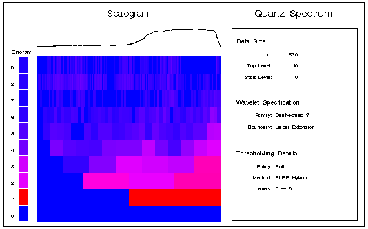
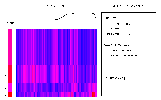
The bar on the left-hand side of the scalogram plot indicates the overall energy of each level. This energy is defined as the sum of the squares of the detail coefficients for each level. These energies are amplified by using the same algorithm for amplifying the detail coefficient magnitudes. The energy bar in Figure 20.12 shows that higher energies occur at the lower levels whose coefficients capture the gross features of the data. In order to interpret the finer-scale details of the data it is helpful to focus on just the higher levels. The following statement produces a scalogram for levels 6 and higher without using a logarithmic scale for the rectangle heights, and using the default coefficient amplification.
      call scalogram(decomp,&SureShrink,6, , , ,
                     "Quartz Spectrum");
The result is shown in Figure 20.13.
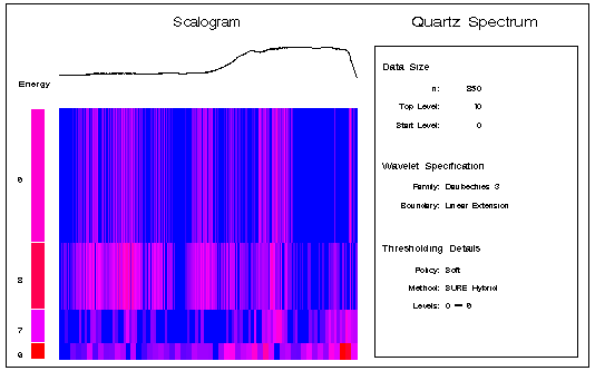
The scalogram in Figure 20.13 reveals that most of the energy of the oscillation in the data is captured in the detail coefficients at level 8. Also note that many of the coefficients at the higher levels are set to zero by "SureShrink" thresholding. You can verify this by comparing Figure 20.13 with Figure 20.14, which shows the corresponding scalogram except that no thresholding is done. The following statement produces Figure 20.14:
call scalogram(decomp, ,6, , , ,"Quartz Spectrum");