Wavelet Analysis

Diagnostic plots greatly facilitate the interpretation of a wavelet decomposition. One standard plot is the detail coefficients arranged by level. By using a module included by the WAVINIT macro call, you can produce the plot shown in Figure 20.5 as follows:
call coefficientPlot(decomp, , , , ,"Quartz Spectrum");
The first argument specifies the wavelet decomposition and is required. All other arguments are optional and need not be specified. You can use the WAVHELP macro to obtain a description of the arguments of this and other wavelet plot modules. The WAVHELP macro is defined in the autocall WAVINIT macro. For example, invoking the WAVHELP macro as follows writes the calling information shown in Figure 20.4 to the SAS log.
%wavhelp(coefficientPlot);
Figure 20.4: Log Output Produced by %wavhelp(coefficientPlot) Call
| coefficientPlot Module |
| Function: Plots wavelet detail coefficients |
| Usage: call coefficientPlot(decomposition, |
| threshopt, |
| startLevel, |
| endLevel, |
| howScaled, |
| header); |
| Arguments: |
| decomposition - (required) valid wavelet decomposition produced |
| by the IML subroutine WAVFT |
| threshopt - (optional) numeric vector of 4 elements |
| specifying thresholding to be used |
| Default: no thresholding |
| startLevel - (optional) numeric scalar specifying the lowest |
| level to be displayed in the plot |
| Default: start level of decomposition |
| endLevel - (optional) numeric scalar specifying the highest |
| level to be displayed in the plot |
| Default: end level of decomposition |
| howScaled - (optional) character: 'absolute' or 'uniform' |
| specifies coefficients are scaled uniformly |
| Default: independent level scaling |
| header - (optional) character string specifying a header |
| Default: no header |
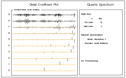
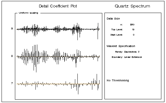
In this plot the detail coefficients at each level are scaled independently. The oscillations present in the absorbance data are captured in the detail coefficients at levels 7, 8, and 9. The following statement produces a coefficient plot of just these higher-level detail coefficients and shows them scaled uniformly.
      call coefficientPlot(decomp, ,7, ,
                           'uniform',"Quartz Spectrum");
The plot is shown in Figure 20.6.
As noted earlier, noise in the data is captured in the detail coefficients, particularly in the small coefficients at higher levels in the decomposition. By zeroing or shrinking these coefficients, you can get smoother reconstructions of the input data. This is done by specifying a threshold value for each level of detail coefficients and then zeroing or shrinking all the detail coefficients below this threshold value. The IML wavelet functions and modules support several policies for how this thresholding is performed as well as for selecting the thresholding value at each level. See the section WAVIFT Call for details.
An options vector is used to specify the desired thresholding; several standard choices are predefined as macro variables in the WAVINIT module. The following statements produce the detail coefficient plot with the "SureShrink" thresholding algorithm of Donoho and Johnstone (1995).
      call coefficientPlot(decomp,&SureShrink,6,, ,
                           "Quartz Spectrum");
The plot is shown in Figure 20.7.
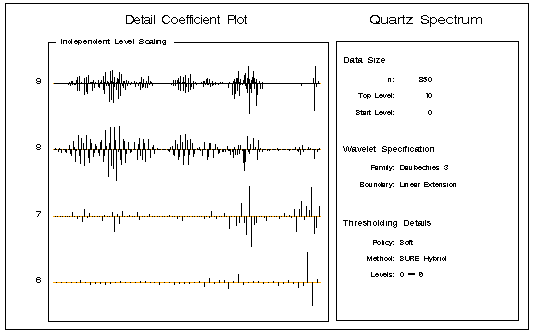
You can see that "SureShrink" thresholding has zeroed some of the detail coefficients at the higher levels but the larger coefficients that capture the oscillation in the data are still present. Consequently, reconstructions of the input signal using the thresholded detail coefficients still capture the essential features of the data, but are smoother because much of the very fine scale detail has been eliminated.