Example 12.4 Brainlog Data
The following data are the body weights (in kilograms) and brain weights (in grams) of ![]() animals as reported by Jerison (1973) and as analyzed in Rousseeuw and Leroy (1987). Instead of the original data, the following example uses the logarithms of the measurements of the two variables.
animals as reported by Jerison (1973) and as analyzed in Rousseeuw and Leroy (1987). Instead of the original data, the following example uses the logarithms of the measurements of the two variables.
title "*** Brainlog Data: Do MCD, MVE ***";
aa={ 1.303338E-001  9.084851E-001 ,
     2.6674530         2.6263400  ,
     1.5602650         2.0773680  ,
     1.4418520         2.0606980  ,
  1.703332E-002     7.403627E-001 ,
     4.0681860         1.6989700  ,
     3.4060290         3.6630410  ,
     2.2720740         2.6222140  ,
     2.7168380         2.8162410  ,
     1.0000000         2.0606980  ,
  5.185139E-001        1.4082400  ,
     2.7234560         2.8325090  ,
     2.3159700         2.6085260  ,
     1.7923920         3.1205740  ,
     3.8230830         3.7567880  ,
     3.9731280         1.8450980  ,
  8.325089E-001        2.2528530  ,
     1.5440680         1.7481880  ,
 -9.208187E-001         .0000000  ,
    -1.6382720     -3.979400E-001 ,
  3.979400E-001        1.0827850  ,
     1.7442930         2.2430380  ,
     2.0000000         2.1959000  ,
     1.7173380         2.6434530  ,
     4.9395190         2.1889280  ,
 -5.528420E-001     2.787536E-001 ,
 -9.136401E-001     4.771213E-001 ,
     2.2833010         2.2552720  };
By default, the MVE subroutine uses only 1500 randomly selected subsets rather than all subsets. The following specification of the options vector requires that all 3276 subsets of 3 cases out of 28 cases are generated and evaluated:
title2 "***MVE for BrainLog Data***";
title3 "*** Use All Subsets***";
optn = j(9,1,.);
optn[1]= 3;              /* ipri */
optn[2]= 1;              /* pcov: print COV */
optn[3]= 1;              /* pcor: print CORR */
optn[5]= -1;             /* nrep: all subsets */

call mve(sc,xmve,dist,optn,aa);
Specifying OPTN[1]=3, OPTN[2]=1, and OPTN[3]=1 requests that all output be printed. Output 12.4.1 shows the classical scatter and correlation matrix.
Output 12.4.1: Some Simple Statistics
| *** Brainlog Data: Do MCD, MVE *** |
| ***MVE for BrainLog Data*** |
| *** Use All Subsets*** |
| Classical Covariance Matrix | ||
|---|---|---|
| VAR1 | VAR2 | |
| VAR1 | 2.6816512357 | 1.3300846932 |
| VAR2 | 1.3300846932 | 1.0857537552 |
| Classical Correlation Matrix | ||
|---|---|---|
| VAR1 | VAR2 | |
| VAR1 | 1 | 0.7794934643 |
| VAR2 | 0.7794934643 | 1 |
| Classical Mean | |
|---|---|
| VAR1 | 1.6378572186 |
| VAR2 | 1.9219465964 |
Output 12.4.2 shows the results of the combinatoric optimization (complete subset sampling).
Output 12.4.2: Iteration History for MVE
| Subset | Singular | Best Criterion |
Percent |
|---|---|---|---|
| 819 | 0 | 0.439709 | 25 |
| 1638 | 0 | 0.439709 | 50 |
| 2457 | 0 | 0.439709 | 75 |
| 3276 | 0 | 0.439709 | 100 |
| Observations of Best Subset | ||
|---|---|---|
| 1 | 22 | 28 |
| Initial MVE Location Estimates |
|
|---|---|
| VAR1 | 1.3859759333 |
| VAR2 | 1.8022650333 |
| Initial MVE Scatter Matrix | ||
|---|---|---|
| VAR1 | VAR2 | |
| VAR1 | 4.9018525125 | 3.2937139101 |
| VAR2 | 3.2937139101 | 2.3400650932 |
Output 12.4.3 shows the optimization results after local improvement.
Output 12.4.3: Table of MVE Results
| Robust MVE Location Estimates | |
|---|---|
| VAR1 | 1.29528238 |
| VAR2 | 1.8733722792 |
| Robust MVE Scatter Matrix | ||
|---|---|---|
| VAR1 | VAR2 | |
| VAR1 | 2.0566592937 | 1.5290250167 |
| VAR2 | 1.5290250167 | 1.2041353589 |
| Eigenvalues of Robust Scatter Matrix |
|
|---|---|
| VAR1 | 3.2177274012 |
| VAR2 | 0.0430672514 |
| Robust Correlation Matrix | ||
|---|---|---|
| VAR1 | VAR2 | |
| VAR1 | 1 | 0.9716184659 |
| VAR2 | 0.9716184659 | 1 |
Output 12.4.4 presents a table that contains the classical Mahalanobis distances, the robust distances, and the weights identifying the outlier observations.
Output 12.4.4: Mahalanobis and Robust Distances
| Classical Distances and Robust (Rousseeuw) Distances | |||
|---|---|---|---|
| Unsquared Mahalanobis Distance and | |||
| Unsquared Rousseeuw Distance of Each Observation | |||
| N | Mahalanobis Distances | Robust Distances | Weight |
| 1 | 1.006591 | 0.897076 | 1.000000 |
| 2 | 0.695261 | 1.405302 | 1.000000 |
| 3 | 0.300831 | 0.186726 | 1.000000 |
| 4 | 0.380817 | 0.318701 | 1.000000 |
| 5 | 1.146485 | 1.135697 | 1.000000 |
| 6 | 2.644176 | 8.828036 | 0 |
| 7 | 1.708334 | 1.699233 | 1.000000 |
| 8 | 0.706522 | 0.686680 | 1.000000 |
| 9 | 0.858404 | 1.084163 | 1.000000 |
| 10 | 0.798698 | 1.580835 | 1.000000 |
| 11 | 0.686485 | 0.693346 | 1.000000 |
| 12 | 0.874349 | 1.071492 | 1.000000 |
| 13 | 0.677791 | 0.717545 | 1.000000 |
| 14 | 1.721526 | 3.398698 | 0 |
| 15 | 1.761947 | 1.762703 | 1.000000 |
| 16 | 2.369473 | 7.999472 | 0 |
| 17 | 1.222253 | 2.805954 | 0 |
| 18 | 0.203178 | 1.207332 | 1.000000 |
| 19 | 1.855201 | 1.773317 | 1.000000 |
| 20 | 2.266268 | 2.074971 | 1.000000 |
| 21 | 0.831416 | 0.785954 | 1.000000 |
| 22 | 0.416158 | 0.342200 | 1.000000 |
| 23 | 0.264182 | 0.918383 | 1.000000 |
| 24 | 1.046120 | 1.782334 | 1.000000 |
| 25 | 2.911101 | 9.565443 | 0 |
| 26 | 1.586458 | 1.543748 | 1.000000 |
| 27 | 1.582124 | 1.808423 | 1.000000 |
| 28 | 0.394664 | 1.523235 | 1.000000 |
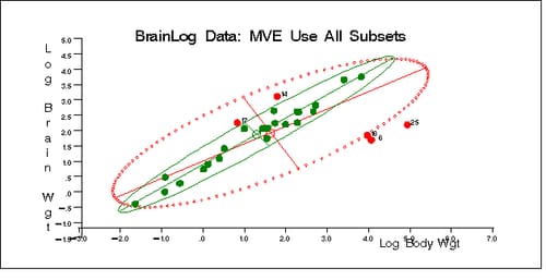
Again, you can call the subroutine SCATMVE(), which is included in the sample library in the file robustmc.sas, to plot the classical and robust confidence ellipsoids, as follows:
optn = j(9,1,.); optn[5]= -1;
vnam = { "Log Body Wgt","Log Brain Wgt" };
filn = "brlmve";
titl = "BrainLog Data: MVE Use All Subsets";
%include 'robustmc.sas';
call scatmve(2,optn,.9,aa,vnam,titl,1,filn);
The plot is shown in Output 12.4.5.
Output 12.4.5: BrainLog Data: Classical and Robust Ellipsoid(MVE)
MCD is another subroutine that can be used to compute the robust location and the robust covariance of multivariate data sets. Here is the code:
title "*** Brainlog Data: Do MCD, MVE ***";
aa={ 1.303338E-001  9.084851E-001 ,
     2.6674530         2.6263400  ,
     1.5602650         2.0773680  ,
     1.4418520         2.0606980  ,
  1.703332E-002     7.403627E-001 ,
     4.0681860         1.6989700  ,
     3.4060290         3.6630410  ,
     2.2720740         2.6222140  ,
     2.7168380         2.8162410  ,
     1.0000000         2.0606980  ,
  5.185139E-001        1.4082400  ,
     2.7234560         2.8325090  ,
     2.3159700         2.6085260  ,
     1.7923920         3.1205740  ,
     3.8230830         3.7567880  ,
     3.9731280         1.8450980  ,
  8.325089E-001        2.2528530  ,
     1.5440680         1.7481880  ,
 -9.208187E-001         .0000000  ,
    -1.6382720     -3.979400E-001 ,
  3.979400E-001        1.0827850  ,
     1.7442930         2.2430380  ,
     2.0000000         2.1959000  ,
     1.7173380         2.6434530  ,
     4.9395190         2.1889280  ,
 -5.528420E-001     2.787536E-001 ,
 -9.136401E-001     4.771213E-001 ,
     2.2833010         2.2552720  };
title2 "***MCD for BrainLog Data***";
title3 "*** Use 500 Random Subsets***";
optn = j(9,1,.);
optn[1]= 3;              /* ipri */
optn[2]= 1;              /* pcov: print COV  */
optn[3]= 1;              /* pcor: print CORR */

call mcd(sc,xmve,dist,optn,aa);
Similarly, specifying OPTN[1]=3, OPTN[2]=1, and OPTN[3]=1 requests that all output be printed.
Output 12.4.6 shows the results of the optimization.
Output 12.4.6: Results of the Optimization
| *** Brainlog Data: Do MCD, MVE *** |
| ***MCD for BrainLog Data*** |
| *** Use 500 Random Subsets*** |
| 1 | 2 | 3 | 4 | 5 | 8 | 9 | 11 | 12 | 13 | 18 | 21 | 22 | 23 | 28 |
| MCD Location Estimate | |
|---|---|
| VAR1 | VAR2 |
| 1.622226068 | 2.0150777867 |
| MCD Scatter Matrix Estimate | ||
|---|---|---|
| VAR1 | VAR2 | |
| VAR1 | 0.8973945995 | 0.6424456706 |
| VAR2 | 0.6424456706 | 0.4793505736 |
Output 12.4.7 shows the reweighted results after removing outliers.
Output 12.4.7: Final Reweighted MCD Results
| Reweighted Location Estimate | |
|---|---|
| VAR1 | VAR2 |
| 1.3154029661 | 1.8568731174 |
| Reweighted Scatter Matrix | ||
|---|---|---|
| VAR1 | VAR2 | |
| VAR1 | 2.139986054 | 1.6068556533 |
| VAR2 | 1.6068556533 | 1.2520384784 |
| Eigenvalues | |
|---|---|
| VAR1 | VAR2 |
| 3.363074897 | 0.0289496354 |
| Reweighted Correlation Matrix | ||
|---|---|---|
| VAR1 | VAR2 | |
| VAR1 | 1 | 0.9816633012 |
| VAR2 | 0.9816633012 | 1 |
Output 12.4.8 presents a table that contains the classical Mahalanobis distances, the robust distances, and the weights identifying the outlier observations.
Output 12.4.8: Mahalanobis and Robust Distances (MCD)
| Classical Distances and Robust (Rousseeuw) Distances | |||
|---|---|---|---|
| Unsquared Mahalanobis Distance and | |||
| Unsquared Rousseeuw Distance of Each Observation | |||
| N | Mahalanobis Distances | Robust Distances | Weight |
| 1 | 1.006591 | 0.855347 | 1.000000 |
| 2 | 0.695261 | 1.477050 | 1.000000 |
| 3 | 0.300831 | 0.239828 | 1.000000 |
| 4 | 0.380817 | 0.517719 | 1.000000 |
| 5 | 1.146485 | 1.108362 | 1.000000 |
| 6 | 2.644176 | 10.599341 | 0 |
| 7 | 1.708334 | 1.808455 | 1.000000 |
| 8 | 0.706522 | 0.690099 | 1.000000 |
| 9 | 0.858404 | 1.052423 | 1.000000 |
| 10 | 0.798698 | 2.077131 | 1.000000 |
| 11 | 0.686485 | 0.888545 | 1.000000 |
| 12 | 0.874349 | 1.035824 | 1.000000 |
| 13 | 0.677791 | 0.683978 | 1.000000 |
| 14 | 1.721526 | 4.257963 | 0 |
| 15 | 1.761947 | 1.716065 | 1.000000 |
| 16 | 2.369473 | 9.584992 | 0 |
| 17 | 1.222253 | 3.571700 | 0 |
| 18 | 0.203178 | 1.323783 | 1.000000 |
| 19 | 1.855201 | 1.741064 | 1.000000 |
| 20 | 2.266268 | 2.026528 | 1.000000 |
| 21 | 0.831416 | 0.743545 | 1.000000 |
| 22 | 0.416158 | 0.419923 | 1.000000 |
| 23 | 0.264182 | 0.944610 | 1.000000 |
| 24 | 1.046120 | 2.289334 | 1.000000 |
| 25 | 2.911101 | 11.471953 | 0 |
| 26 | 1.586458 | 1.518721 | 1.000000 |
| 27 | 1.582124 | 2.054593 | 1.000000 |
| 28 | 0.394664 | 1.675651 | 1.000000 |
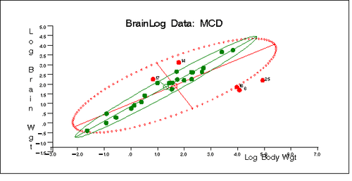
You can call the subroutine SCATMCD(), which is included in the sample library in file robustmc.sas, to plot the classical and robust confidence ellipsoids. Here is the code:
optn = j(9,1,.); optn[5]= -1;
vnam = { "Log Body Wgt","Log Brain Wgt" };
filn = "brlmcd";
titl = "BrainLog Data: MCD";
%include 'robustmc.sas';
call scatmcd(2,optn,.9,aa,vnam,titl,1,filn);
The plot is shown in Output 12.4.9.
Output 12.4.9: BrainLog Data: Classical and Robust Ellipsoid (MCD)