Example 13.1 VAR Estimation and Variance Decomposition
In this example, a VAR model is estimated and forecast. The VAR(3) model is estimated by using investment, durable consumption, and consumption expenditures. The data are found in the appendix to Lütkepohl (1993). The stationary VAR(3) process is specified as
The matrix ARCOEF contains the AR coefficients ( ,
, , and
, and  ), and the matrix EV contains error covariance estimates. An intercept vector
  is included in the first row of the matrix ARCOEF if OPT[1]=1 is specified. Here is the code:
   data one;
      input invest income consum @@;
   datalines;
   180 451  415  179 465  421   185 485  434   192 493  448
   211 509  459  202 520  458   207 521  479   214 540  487
   231 548  497  229 558  510   234 574  516   237 583  525
   206 591  529  250 599  538   259 610  546   263 627  555
   264 642  574  280 653  574   282 660  586   292 694  602
   286 709  617  302 734  639   304 751  653   307 763  668
   317 766  679  314 779  686   306 808  697   304 785  688
   292 794  704  275 799  699   273 799  709   301 812  715
   280 837  724  289 853  746   303 876  758   322 897  779
   315 922  798  339 949  816   364 979  837   371 988  858
   375 1025 881  432 1063 905   453 1104 934   460 1131 968
   475 1137 983  496 1178 1013  494 1211 1034  498 1256 1064
   526 1290 1101 519 1314 1102  516 1346 1145  531 1385 1173
   573 1416 1216 551 1436 1229  538 1462 1242  532 1493 1267
   558 1516 1295 524 1557 1317  525 1613 1355  519 1642 1371
   526 1690 1402 510 1759 1452  519 1756 1485  538 1780 1516
   549 1807 1549 570 1831 1567  559 1873 1588  584 1897 1631
   611 1910 1650 597 1943 1685  603 1976 1722  619 2018 1752
   635 2040 1774 658 2070 1807  675 2121 1831  700 2132 1842
   692 2199 1890 759 2253 1958  782 2276 1948  816 2318 1994
   844 2369 2061 830 2423 2056  853 2457 2102  852 2470 2121
   833 2521 2145 860 2545 2164  870 2580 2206  830 2620 2225
   801 2639 2235 824 2618 2237  831 2628 2250  830 2651 2271
   ;
   proc iml;
   use one;
   read all into y var{invest income consum};
   mdel  = 1;
   maice = 0;
   misw  = 0;  /*-- instantaneous modeling ? --*/
   call tsmulmar(arcoef,ev,nar,aic) data=y maxlag=3
        opt=(mdel || maice || misw) print=1;
   arcoef = j(9,3,0);
   do i=1 to 9;
      do j=1 to 3;
         arcoef[i,j] = arcoef_l[i+1,j];
      end;
   end;
   print arcoef;
   misw = 1;
   call tsmulmar(arcoef,ev,nar,aic) data=y maxlag=3
           opt=(mdel || maice || misw) print=1;
   print ev;
To obtain the unit triangular matrix  and diagonal matrix
  , you need to estimate the instantaneous response model. When you specify the OPT[3]=1 option, the first row of the output matrix EV contains error variances of the instantaneous response model, while the unit triangular matrix is in the second through the fifth rows. See Output 13.1.1. Here is the code:
Output 13.1.1
Error Variance and Unit Triangular Matrix
| VAR Estimation and Variance Decomposition |
| 295.21042 |
190.94664 |
59.361516 |
| 1 |
0 |
0 |
| -0.02239 |
1 |
0 |
| -0.256341 |
-0.500803 |
1 |
In Output 13.1.2 and Output 13.1.3, you can see the relationship between the instantaneous response model and the VAR model. The VAR coefficients are computed as  , where
  is a coefficient matrix of the instantaneous model. For example, you can verify this result by using the first lag coefficient matrix
  .
.
   proc iml;
   mdel  = 1;
   maice = 0;
   misw  = 0;
   call tsmulmar(arcoef,ev,nar,aic) data=y maxlag=3
        opt=(mdel || maice || misw);
   call tspred(forecast,impulse0,mse,y,arcoef,nar,0,ev)
        npred=10 start=nrow(y) constant=mdel;
Output 13.1.2
VAR Estimates
| 0.8855926 |
0.3401741 |
-0.014398 |
| 0.1684523 |
1.0502619 |
0.107064 |
| 0.0891034 |
0.4591573 |
0.4473672 |
| -0.059195 |
-0.298777 |
0.1629818 |
| 0.1128625 |
-0.044039 |
-0.088186 |
| 0.1684932 |
-0.025847 |
-0.025671 |
| 0.0637227 |
-0.196504 |
0.0695746 |
| -0.226559 |
0.0532467 |
-0.099808 |
| -0.303697 |
-0.139022 |
0.2576405 |
Output 13.1.3
Instantaneous Response Model Estimates
| 0.885593 |
0.340174 |
-0.014398 |
| 0.148624 |
1.042645 |
0.107386 |
| -0.222272 |
-0.154018 |
0.39744 |
| -0.059195 |
-0.298777 |
0.162982 |
| 0.114188 |
-0.037349 |
-0.091835 |
| 0.127145 |
0.072796 |
-0.023287 |
| 0.063723 |
-0.196504 |
0.069575 |
| -0.227986 |
0.057646 |
-0.101366 |
| -0.20657 |
-0.115316 |
0.28979 |
When the VAR estimates are available, you can forecast the future values by using the TSPRED call. As a default, the one-step predictions are produced until the START= point is reached. The NPRED= option specifies how far you want to predict. The prediction error covariance matrix MSE contains mean square error matrices. The output matrix IMPULSE contains the estimate of the coefficients
  of the infinite MA process. The following IML code estimates the VAR(3) model and performs 10-step-ahead prediction.
   mdel  = 1;
   maice = 0;
   misw  = 0;
   call tsmulmar(arcoef,ev,nar,aic) data=y maxlag=3
        opt=(mdel || maice || misw);
   call tspred(forecast,impulse,mse,y,arcoef,nar,0,ev)
        npred=10 start=nrow(y) constant=mdel;
   print impulse;
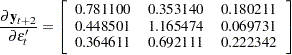
The lagged effects of a unit increase in the error disturbances are included in the matrix IMPULSE. For example:
Output 13.1.4 displays the first 15 rows of the matrix IMPULSE.
Output 13.1.4
Moving-Average Coefficients: MA(0) MA(4)
MA(4)
| 1 |
0 |
0 |
| 0 |
1 |
0 |
| 0 |
0 |
1 |
| 0.8855926 |
0.3401741 |
-0.014398 |
| 0.1684523 |
1.0502619 |
0.107064 |
| 0.0891034 |
0.4591573 |
0.4473672 |
| 0.7810999 |
0.3531397 |
0.1802109 |
| 0.4485013 |
1.1654737 |
0.0697311 |
| 0.3646106 |
0.6921108 |
0.2223425 |
| 0.8145483 |
0.243637 |
0.2914643 |
| 0.4997732 |
1.3625363 |
-0.018202 |
| 0.2775237 |
0.7555914 |
0.3885065 |
| 0.7960884 |
0.2593068 |
0.260239 |
| 0.5275069 |
1.4134792 |
0.0335483 |
| 0.267452 |
0.8659426 |
0.3190203 |
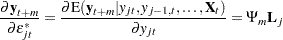
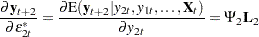
In addition, you can compute the lagged response on the one-unit increase in the orthogonalized disturbances  .
.
When the error matrix EV is obtained from the instantaneous response model, you need to convert the matrix IMPULSE. The first 15 rows of the matrix ORTH_IMP are shown in Output 13.1.5. Note that the matrix constructed from the last three rows of EV become the matrix . Here is the code:
   call tsmulmar(arcoef,ev,nar,aic) data=y maxlag=3
        opt={1 0 1};
   lmtx = inv(ev[2:nrow(ev),]);
   orth_imp = impulse * lmtx;
   print orth_imp;
Output 13.1.5
Transformed Moving-Average Coefficients
| 1 |
0 |
0 |
| 0.0223902 |
1 |
0 |
| 0.267554 |
0.5008031 |
1 |
| 0.889357 |
0.3329638 |
-0.014398 |
| 0.2206132 |
1.1038799 |
0.107064 |
| 0.219079 |
0.6832001 |
0.4473672 |
| 0.8372229 |
0.4433899 |
0.1802109 |
| 0.4932533 |
1.2003953 |
0.0697311 |
| 0.4395957 |
0.8034606 |
0.2223425 |
| 0.8979858 |
0.3896033 |
0.2914643 |
| 0.5254106 |
1.3534206 |
-0.018202 |
| 0.398388 |
0.9501566 |
0.3885065 |
| 0.8715223 |
0.3896353 |
0.260239 |
| 0.5681309 |
1.4302804 |
0.0335483 |
| 0.3721958 |
1.025709 |
0.3190203 |
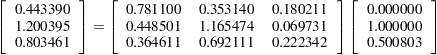
You can verify the result for the case of
using the simple computation
The contribution of the  th orthogonalized innovation to the mean square error matrix of the 10-step forecast is computed by using the formula
In Output 13.1.6, diagonal elements of each decomposed MSE matrix are displayed as the matrix CONTRIB as well as those of the MSE matrix (VAR). Here is the code:
   mse1  = j(3,3,0);
   mse2  = j(3,3,0);
   mse3  = j(3,3,0);
   do i = 1 to 5;
      psi = impulse[(i-1)*3+1:3*i,];
      mse1 = mse1 + psi*lmtx[,1]*lmtx[,1]`*psi`;
      mse2 = mse2 + psi*lmtx[,2]*lmtx[,2]`*psi`;
      mse3 = mse3 + psi*lmtx[,3]*lmtx[,3]`*psi`;
   end;
   mse1 = ev[1,1]#mse1;
   mse2 = ev[1,2]#mse2;
   mse3 = ev[1,3]#mse3;
   contrib = vecdiag(mse1) || vecdiag(mse2) || vecdiag(mse3);
   var  = vecdiag(mse[28:30,]);
   print contrib var;
Output 13.1.6
Orthogonal Innovation Contribution
| 1197.9131 |
116.68096 |
11.003194 |
2163.7104 |
| 263.12088 |
1439.1551 |
1.0555626 |
4573.9809 |
| 180.09836 |
633.55931 |
89.177905 |
2466.506 |
The investment innovation contribution to its own variable is 1879.3774, and the income innovation contribution to the consumption expenditure is 1916.1676. It is easy to understand the contribution of innovations in the th variable to MSE when you compute the innovation account. In Output 13.1.7, innovations in the first variable (investment) explain 20.45% of the error variance of the second variable (income), while the innovations in the second variable explain 79.5% of its own error variance. It is straightforward to construct the general multistep forecast error variance decomposition. Here is the code:
   account = contrib * 100 / (var@j(1,3,1));
   print account;
Output 13.1.7
Innovation Account
| 55.363835 |
5.3926331 |
0.5085336 |
| 5.7525574 |
31.463951 |
0.0230775 |
| 7.3017604 |
25.68651 |
3.615556 |