Minimum AIC Procedure

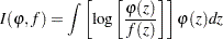
The AIC statistic is widely used to select the best model among alternative parametric models. The minimum AIC model selection procedure can be interpreted as a maximization of the expected entropy (Akaike; 1981). The entropy of a true probability density function (PDF) with respect to the fitted PDF is written as

where is a Kullback-Leibler information measure, which is defined as

where the random variable is assumed to be continuous. Therefore,

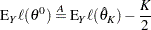
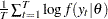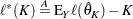
where and E denotes the expectation concerning the random variable . if and only if (a.s.). The larger the quantity E, the closer the function is to the true PDF . Given the data that has the same distribution as the random variable , let the likelihood function of the parameter vector be . Then the average of the log-likelihood function is an estimate of the expected value of . Akaike (1981) derived the alternative estimate of E by using the Bayesian predictive likelihood. The AIC is the bias-corrected estimate of 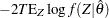, where is the maximum likelihood estimate.

Let be a parameter vector that is contained in the parameter space . Given the data , the log-likelihood function is

Suppose the probability density function has the true PDF , where the true parameter vector is contained in . Let be a maximum likelihood estimate. The maximum of the log-likelihood function is denoted as . The expected log-likelihood function is defined by

The Taylor series expansion of the expected log-likelihood function around the true parameter gives the following asymptotic relationship:

where is the information matrix and stands for asymptotic equality. Note that since is maximized at . By substituting , the expected log-likelihood function can be written as

The maximum likelihood estimator is asymptotically normally distributed under the regularity conditions

Therefore,

The mean expected log-likelihood function, , becomes

When the Taylor series expansion of the log-likelihood function around is used, the log-likelihood function is written

Since is the maximum log-likelihood function, . Note that if the maximum likelihood estimator is a consistent estimator of . Replacing with the true parameter and taking expectations with respect to the random variable ,

Consider the following relationship:

From the previous derivation,

Therefore,

The natural estimator for E is . Using this estimator, you can write the mean expected log-likelihood function as

Consequently, the AIC is defined as an asymptotically unbiased estimator of

In practice, the previous asymptotic result is expected to be valid in finite samples if the number of free parameters does not exceed and the upper bound of the number of free parameters is . It is worth noting that the amount of AIC is not meaningful in itself, since this value is not the Kullback-Leibler information measure. The difference of AIC values can be used to select the model. The difference of the two AIC values is considered insignificant if it is far less than 1. It is possible to find a better model when the minimum AIC model contains many free parameters.

Smoothness Priors Modeling

Consider the time series :

where is an unknown smooth function and is an random variable with zero mean and positive variance . Whittaker (1923) provides the solution, which balances a tradeoff between closeness to the data and the th-order difference equation. For a fixed value of and , the solution satisfies

where denotes the th-order difference operator. The value of can be viewed as the smoothness tradeoff measure. Akaike (1980a) proposed the Bayesian posterior PDF to solve this problem.

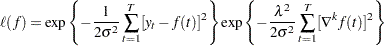Therefore, the solution can be obtained when the function is maximized.

Assume that time series is decomposed as follows:

where denotes the trend component and is the seasonal component. The trend component follows the th-order stochastically perturbed difference equation.

For example, the polynomial trend component for is written as

To accommodate regular seasonal effects, the stochastic seasonal relationship is used.

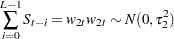where is the number of seasons within a period. In the context of Whittaker and Akaike, the smoothness priors problem can be solved by the maximization of

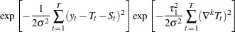The values of hyperparameters and refer to a measure of uncertainty of prior information. For example, the large value of implies a relatively smooth trend component. The ratio can be considered as a signal-to-noise ratio.

Kitagawa and Gersch (1984) use the Kalman filter recursive computation for the likelihood of the tradeoff parameters. The hyperparameters are estimated by combining the grid search and optimization method. The state space model and Kalman filter recursive computation are discussed in the section State Space and Kalman Filter Method.

Bayesian Seasonal Adjustment

Seasonal phenomena are frequently observed in many economic and business time series. For example, consumption expenditure might have strong seasonal variations because of Christmas spending. The seasonal phenomena are repeatedly observed after a regular period of time. The number of seasons within a period is defined as the smallest time span for this repetitive observation. Monthly consumption expenditure shows a strong increase during the Christmas season, with 12 seasons per period.

There are three major approaches to seasonal time series: the regression model, the moving average model, and the seasonal ARIMA model.

Regression Model

Let the trend component be and the seasonal component be
. Then the additive time series can be written as the regression model

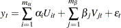In practice, the trend component can be written as the th-order polynomial, such as

The seasonal component can be approximated by the seasonal dummies

where is the number of seasons within a period. The least squares method is applied to estimate parameters and .

The seasonally adjusted series is obtained by subtracting the estimated seasonal component from the original series. Usually, the error term is assumed to be white noise, while sometimes the autocorrelation of the regression residuals needs to be allowed. However, the regression method is not robust to the regression function type, especially at the beginning and end of the series.

Moving Average Model

If you assume that the annual sum of a seasonal time series has small seasonal fluctuations, the nonseasonal component can be estimated by using the moving average method.

where is the positive integer and is the symmetric constant such that and .

When the data are not available, either an asymmetric moving average is used, or the forecast data are augmented to use the symmetric weight. The X-11 procedure is a complex modification of this moving-average method.

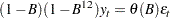
Seasonal ARIMA Model

The regression and moving-average approaches assume that the seasonal component is deterministic and independent of other nonseasonal components. The time series approach is used to handle the stochastic trend and seasonal components.

The general ARIMA model can be written

where is the backshift operator and

and if ; otherwise, . The power of , , can be considered as a seasonal factor. Specifically, the Box-Jenkins multiplicative seasonal ARIMA model is written as

ARIMA modeling is appropriate for particular time series and requires burdensome computation.

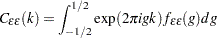
The TSBAYSEA subroutine combines the simple characteristics of the regression approach and time series modeling. The TSBAYSEA and X-11 procedures use the model-based seasonal adjustment. The symmetric weights of the standard X-11 option can be approximated by using the integrated MA form

With a fixed value , the TSBAYSEA subroutine is approximated as

The subroutine is flexible enough to handle trading-day or leap-year effects, the shift of the base observation, and missing values. The TSBAYSEA-type modeling approach has some advantages: it clearly defines the statistical model of the time series; modification of the basic model can be an efficient method of choosing a particular procedure for the seasonal adjustment of a given time series; and the use of the concept of the likelihood provides a minimum AIC model selection approach.

Nonstationary Time Series

The subroutines TSMLOCAR, TSMLOMAR, and TSTVCAR are used to analyze nonstationary time series models. The AIC statistic is extensively used to analyze the locally stationary model.

Locally Stationary AR Model

When the time series is nonstationary, the TSMLOCAR (univariate) and TSMLOMAR (multivariate) subroutines can be employed. The whole span of the series is divided into locally stationary blocks of data, and then the TSMLOCAR and TSMLOMAR subroutines estimate a stationary AR model by using the least squares method on this stationary block. The homogeneity of two different blocks of data is tested by using the AIC.

Given a set of data , the data can be divided into blocks of sizes , where , and and are unknown. The locally stationary model is fitted to the data

where

where is a Gaussian white noise with and . Therefore, the log-likelihood function of the locally stationary series is

Given , , the maximum of the log-likelihood function is attained at

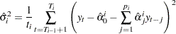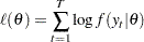
The concentrated log-likelihood function is given by

Therefore, the maximum likelihood estimates, and , are obtained by minimizing the following local SSE:

The least squares estimation of the stationary model is explained in the section Least Squares and Householder Transformation.

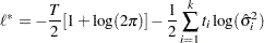
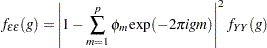
The AIC for the locally stationary model over the pooled data is written as

where intercept = 1 if the intercept term is estimated; otherwise, intercept = 0. The number of stationary blocks (), the size of each block (), and the order of the locally stationary model is determined by the AIC. Consider the autoregressive model fitted over the block of data, , and let this model be an AR() process. When additional data, , are available, a new model , an AR() process, is fitted over this new data set, assuming that these data are independent of the previous data. Then AICs for models and are defined as

The joint model AIC for and is obtained by summation

When the two data sets are pooled and estimated over the pooled data set, , the AIC of the pooled model is

where is the pooled error variance and is the order chosen to fit the pooled data set.

Decision

• If , switch to the new model, since there is a change in the structure of the time series.

• If , pool the two data sets, since two data sets are considered to be homogeneous.

If new observations are available, repeat the preceding steps to determine the homogeneity of the data. The basic idea of locally stationary AR modeling is that, if the structure of the time series is not changed, you should use the additional information to improve the model fitting, but you need to follow the new structure of the time series if there is any change.

Time-Varying AR Coefficient Model

Another approach to nonstationary time series, especially those that are nonstationary in the covariance, is time-varying AR coefficient modeling. When the time series is nonstationary in the covariance, the problem in modeling this series is related to an efficient parameterization. It is possible for a Bayesian approach to estimate the model with a large number of implicit parameters of the complex structure by using a relatively small number of hyperparameters.

The TSTVCAR subroutine uses smoothness priors by imposing stochastically perturbed difference equation constraints on each AR coefficient and frequency response function. The variance of each AR coefficient distribution constitutes a hyperparameter included in the state space model. The likelihood of these hyperparameters is computed by the Kalman filter recursive algorithm.

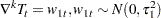
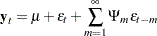
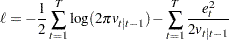
The time-varying AR coefficient model is written

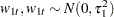
where time-varying coefficients are assumed to change gradually with time. The following simple stochastic difference equation constraint is imposed on each coefficient:

The frequency response function of the AR process is written

The smoothness of this function can be measured by the th derivative smoothness constraint,

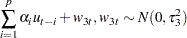
Then the TSTVCAR call imposes zero and second derivative smoothness constraints. The time-varying AR coefficients are the solution of the following constrained least squares:

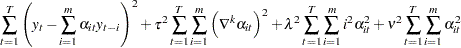where , , and are hyperparameters of the prior distribution.

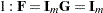
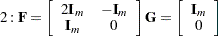
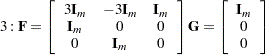
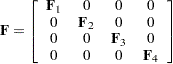
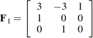
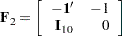
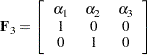
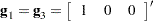
Using a state space representation, the model is

where

The computation of the likelihood function is straightforward. See the section State Space and Kalman Filter Method for the computation method.

Multivariate Time Series Analysis

The subroutines TSMULMAR, TSMLOMAR, and TSPRED analyze multivariate time series. The periodic AR model, TSPEARS, can also be estimated by using a vector AR procedure, since the periodic AR series can be represented as the covariance-stationary vector autoregressive model.

The stationary vector AR model is estimated and the order of the model (or each variable) is automatically determined by the minimum AIC procedure. The stationary vector AR model is written

Using the factorization method, the error covariance is decomposed as

where is a unit lower triangular matrix and is a diagonal matrix. Then the instantaneous response model is defined as

where , for , and . Each equation of the instantaneous response model can be estimated independently, since its error covariance matrix has a diagonal covariance matrix . Maximum likelihood estimates are obtained through the least squares method when the disturbances are normally distributed and the presample values are fixed.

The TSMULMAR subroutine estimates the instantaneous response model. The VAR coefficients are computed by using the relationship between the VAR and instantaneous models.

The general VARMA model can be transformed as an infinite-order MA process under certain conditions.

In the context of the VAR() model, the coefficient can be interpreted as the -lagged response of a unit increase in the disturbances at time .

The lagged response on the one-unit increase in the orthogonalized disturbances is denoted

where is the th column of the unit triangular matrix and . When you estimate the VAR model by using the TSMULMAR call, it is easy to compute this impulse response function.

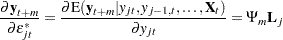
The MSE of the -step prediction is computed as

Note that . Then the covariance matrix of is decomposed

where is the th diagonal element of the matrix and is the number of variables. The MSE matrix can be written

Therefore, the contribution of the th orthogonalized innovation to the MSE is

The th forecast error variance decomposition is obtained from diagonal elements of the matrix .

The nonstationary multivariate series can be analyzed by the TSMLOMAR subroutine. The estimation and model identification procedure is analogous to the univariate nonstationary procedure, which is explained in the section Nonstationary Time Series.

A time series is periodically correlated with period if and . Let be autoregressive of period with AR orders —that is,

where is uncorrelated with mean zero and , , , and . Define the new variable such that . The vector series, , is autoregressive of order , where . The TSPEARS subroutine estimates the periodic autoregressive model by using minimum AIC vector AR modeling.

The TSPRED subroutine computes the one-step or multistep forecast of the multivariate ARMA model if the ARMA parameter estimates are provided. In addition, the subroutine TSPRED produces the (intermediate and permanent) impulse response function and performs forecast error variance decomposition for the vector AR model.

Spectral Analysis

The autocovariance function of the random variable is defined as

where . When the real valued process is stationary and its autocovariance is absolutely summable, the population spectral density function is obtained by using the Fourier transform of the autocovariance function

where and is the autocovariance function such that .

Consider the autocovariance generating function

where and is a complex scalar. The spectral density function can be represented as

The stationary ARMA() process is denoted

where and do not have common roots. Note that the autocovariance generating function of the linear process is given by

For the ARMA() process, . Therefore, the spectral density function of the stationary ARMA() process becomes

The spectral density function of a white noise is a constant.

The spectral density function of the AR(1) process is given by

The spectrum of the AR(1) process has its minimum at and its maximum at if , while the spectral density function attains its maximum at and its minimum at , if . When the series is positively autocorrelated, its spectral density function is dominated by low frequencies. It is interesting to observe that the spectrum approaches as . This relationship shows that the series is difference-stationary if its spectral density function has a remarkable peak near 0.

The spectrum of AR(2) process equals

Refer to Anderson (1971) for details of the characteristics of this spectral density function of the AR(2) process.

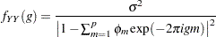
In practice, the population spectral density function cannot be computed. There are many ways of computing the sample spectral density function. The TSBAYSEA and TSMLOCAR subroutines compute the power spectrum by using AR coefficients and the white noise variance.

The power spectral density function of is derived by using the Fourier transformation of .

where and denotes frequency. The autocovariance function can also be written as

Consider the following stationary AR() process:

where is a white noise with mean zero and constant variance .

The autocovariance function of white noise equals

where if ; otherwise, . Therefore, the power spectral density of the white noise is , . Note that, with ,

Using the following autocovariance function of ,

the autocovariance function of the white noise is denoted as

On the other hand, another formula of the gives

Therefore,

Since , the rational spectrum of is

To compute the power spectrum, estimated values of white noise variance and AR coefficients are used. The order of the AR process can be determined by using the minimum AIC procedure.

Computational Details

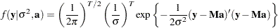
Least Squares and Householder Transformation

Consider the univariate AR() process

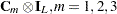
Define the design matrix .

Let . The least squares estimate, , is the approximation to the maximum likelihood estimate of if is assumed to be Gaussian error disturbances. Combining and as

the matrix can be decomposed as

where is an orthogonal matrix and is an upper triangular matrix, , and .

The least squares estimate that uses Householder transformation is computed by solving the linear system

The unbiased residual variance estimate is

and

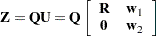
In practice, least squares estimation does not require the orthogonal matrix . The TIMSAC subroutines compute the upper triangular matrix without computing the matrix .

Bayesian Constrained Least Squares

Consider the additive time series model

Practically, it is not possible to estimate parameters , since the number of parameters exceeds the number of available observations. Let denote the seasonal difference operator with seasons and degree of ; that is, . Suppose that . Some constraints on the trend and seasonal components need to be imposed such that the sum of squares of , , and is small. The constrained least squares estimates are obtained by minimizing

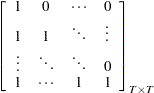
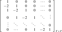
Using matrix notation,

where , , and is the initial guess of . The matrix is a control matrix in which structure varies according to the order of differencing in trend and season.

where

The matrix has the same structure as the matrix , and is the identity matrix. The solution of the constrained least squares method is equivalent to that of maximizing the function

Therefore, the PDF of the data is

The prior PDF of the parameter vector is

When the constant is known, the estimate of is the mean of the posterior distribution, where the posterior PDF of the parameter is proportional to the function . It is obvious that is the minimizer of , where

The value of is determined by the minimum ABIC procedure. The ABIC is defined as

State Space and Kalman Filter Method

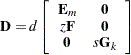
In this section, the mathematical formulas for state space modeling are introduced. The Kalman filter algorithms are derived from the state space model. As an example, the state space model of the TSDECOMP subroutine is formulated.

Define the following state space model:

where and . If the observations, , and the initial conditions, and , are available, the one-step predictor of the state vector and its mean square error (MSE) matrix are written as

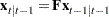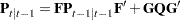Using the current observation, the filtered value of and its variance are updated.

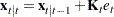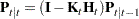where 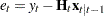and . The log-likelihood function is computed as

where is the conditional variance of the one-step prediction error .

Consider the additive time series decomposition

where is a regressor vector and is a time-varying coefficient vector. Each component has the following constraints:

where and . The AR component is assumed to be stationary. The trading-day component represents the number of the th day of the week in time . If , and (monthly data),

The state vector is defined as

The matrix is

where

The matrix can be denoted as

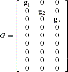where

Finally, the matrix is time-varying,

where

Missing Values

The TIMSAC subroutines skip any missing values at the beginning of the data set. When the univariate and multivariate AR models are estimated via least squares (TSMLOCAR, TSMLOMAR, TSUNIMAR, TSMULMAR, and TSPEARS), there are three options available; that is, MISSING=0, MISSING=1, or MISSING=2. When the MISSING=0 (default) option is specified, the first contiguous observations with no missing values are used. The MISSING=1 option specifies that only nonmissing observations should be used by ignoring the observations with missing values. If the MISSING=2 option is specified, the missing values are filled with the sample mean. The least squares estimator with the MISSING=2 option is biased in general.

The BAYSEA subroutine assumes the same prior distribution of the trend and seasonal components that correspond to the missing observations. A modification is made to skip the components of the vector that correspond to the missing observations. The vector is defined in the section Bayesian Constrained Least Squares. In addition, the TSBAYSEA subroutine considers outliers as missing values. The TSDECOMP and TSTVCAR subroutines skip the Kalman filter updating equation when the current observation is missing.

ISM TIMSAC Packages

A description of each TIMSAC package follows. Each description includes a list of the programs provided in the TIMSAC version.