Getting Started
Unconstrained Rosenbrock Function
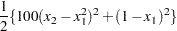
The Rosenbrock function is defined as
 |
 |
 |
|||
 |
|
 |
The minimum function value  is at the point
  .
.
The following code calls the NLPTR subroutine to solve the optimization problem:
The NLPTR is a trust-region optimization method. The F_ROSEN module represents the Rosenbrock function, and the G_ROSEN module represents its gradient. Specifying the gradient can reduce the number of function calls by the optimization subroutine. The optimization begins at the initial point  . For more information about the NLPTR subroutine and its arguments, see the section NLPTR Call. For details about the options vector, which is given by the OPTN vector in the preceding code, see the section Options Vector.
A portion of the output produced by the NLPTR subroutine is shown in Figure 14.1.
| Optimization Start | |||
|---|---|---|---|
| Parameter Estimates | |||
| N | Parameter | Estimate | Gradient Objective Function |
| 1 | X1 | -1.200000 | -107.800000 |
| 2 | X2 | 1.000000 | -44.000000 |
| Parameter Estimates | 2 |
|---|
| Optimization Start | |||
|---|---|---|---|
| Active Constraints | 0 | Objective Function | 12.1 |
| Max Abs Gradient Element | 107.8 | Radius | 1 |
| Iteration | Restarts | Function Calls |
Active Constraints |
Objective Function |
Objective Function Change |
Max Abs Gradient Element |
Lambda | Trust Region Radius |
||
|---|---|---|---|---|---|---|---|---|---|---|
| 1 | 0 | 2 | 0 | 2.36594 | 9.7341 | 2.3189 | 0 | 1.000 | ||
| 2 | 0 | 5 | 0 | 2.05926 | 0.3067 | 5.2875 | 0.385 | 1.526 | ||
| 3 | 0 | 8 | 0 | 1.74390 | 0.3154 | 5.9934 | 0 | 1.086 | ||
| 4 | 0 | 9 | 0 | 1.43279 | 0.3111 | 6.5134 | 0.918 | 0.372 | ||
| 5 | 0 | 10 | 0 | 1.13242 | 0.3004 | 4.9245 | 0 | 0.373 | ||
| 6 | 0 | 11 | 0 | 0.86905 | 0.2634 | 2.9302 | 0 | 0.291 | ||
| 7 | 0 | 12 | 0 | 0.66711 | 0.2019 | 3.6584 | 0 | 0.205 | ||
| 8 | 0 | 13 | 0 | 0.47959 | 0.1875 | 1.7354 | 0 | 0.208 | ||
| 9 | 0 | 14 | 0 | 0.36337 | 0.1162 | 1.7589 | 2.916 | 0.132 | ||
| 10 | 0 | 15 | 0 | 0.26903 | 0.0943 | 3.4089 | 0 | 0.270 | ||
| 11 | 0 | 16 | 0 | 0.16280 | 0.1062 | 0.6902 | 0 | 0.201 | ||
| 12 | 0 | 19 | 0 | 0.11590 | 0.0469 | 1.1456 | 0 | 0.316 | ||
| 13 | 0 | 20 | 0 | 0.07616 | 0.0397 | 0.8462 | 0.931 | 0.134 | ||
| 14 | 0 | 21 | 0 | 0.04873 | 0.0274 | 2.8063 | 0 | 0.276 | ||
| 15 | 0 | 22 | 0 | 0.01862 | 0.0301 | 0.2290 | 0 | 0.232 | ||
| 16 | 0 | 25 | 0 | 0.01005 | 0.00858 | 0.4553 | 0 | 0.256 | ||
| 17 | 0 | 26 | 0 | 0.00414 | 0.00590 | 0.4297 | 0.247 | 0.104 | ||
| 18 | 0 | 27 | 0 | 0.00100 | 0.00314 | 0.4323 | 0.0453 | 0.104 | ||
| 19 | 0 | 28 | 0 | 0.0000961 | 0.000906 | 0.1134 | 0 | 0.104 | ||
| 20 | 0 | 29 | 0 | 1.67875E-6 | 0.000094 | 0.0224 | 0 | 0.0569 | ||
| 21 | 0 | 30 | 0 | 6.9583E-10 | 1.678E-6 | 0.000336 | 0 | 0.0248 | ||
| 22 | 0 | 31 | 0 | 1.3128E-16 | 6.96E-10 | 1.977E-7 | 0 | 0.00314 |
| Optimization Results | |||
|---|---|---|---|
| Iterations | 22 | Function Calls | 32 |
| Hessian Calls | 23 | Active Constraints | 0 |
| Objective Function | 1.312819E-16 | Max Abs Gradient Element | 1.9773301E-7 |
| Lambda | 0 | Actual Over Pred Change | 0 |
| Radius | 0.0031402097 | ||
| ABSGCONV convergence criterion satisfied. |
| Optimization Results | |||
|---|---|---|---|
| Parameter Estimates | |||
| N | Parameter | Estimate | Gradient Objective Function |
| 1 | X1 | 1.000000 | 0.000000198 |
| 2 | X2 | 1.000000 | -0.000000105 |
Since 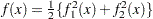 , you can also use least squares techniques in this situation. The following code calls the NLPLM subroutine to solve the problem. The output is shown in Figure 14.2.
| Optimization Start | |||
|---|---|---|---|
| Parameter Estimates | |||
| N | Parameter | Estimate | Gradient Objective Function |
| 1 | X1 | -1.200000 | -107.799999 |
| 2 | X2 | 1.000000 | -44.000000 |
| Parameter Estimates | 2 |
|---|---|
| Functions (Observations) | 2 |
| Optimization Start | |||
|---|---|---|---|
| Active Constraints | 0 | Objective Function | 12.1 |
| Max Abs Gradient Element | 107.79999885 | Radius | 2626.5613241 |
| Iteration | Restarts | Function Calls |
Active Constraints |
Objective Function |
Objective Function Change |
Max Abs Gradient Element |
Lambda | Ratio Between Actual and Predicted Change |
||
|---|---|---|---|---|---|---|---|---|---|---|
| 1 | 0 | 4 | 0 | 2.18185 | 9.9181 | 17.4704 | 0.00804 | 0.964 | ||
| 2 | 0 | 6 | 0 | 1.59370 | 0.5881 | 3.7015 | 0.0190 | 0.988 | ||
| 3 | 0 | 7 | 0 | 1.32848 | 0.2652 | 7.0843 | 0.00830 | 0.678 | ||
| 4 | 0 | 8 | 0 | 1.03891 | 0.2896 | 6.3092 | 0.00753 | 0.593 | ||
| 5 | 0 | 9 | 0 | 0.78943 | 0.2495 | 7.2617 | 0.00634 | 0.486 | ||
| 6 | 0 | 10 | 0 | 0.58838 | 0.2011 | 7.8837 | 0.00462 | 0.393 | ||
| 7 | 0 | 11 | 0 | 0.34224 | 0.2461 | 6.6815 | 0.00307 | 0.524 | ||
| 8 | 0 | 12 | 0 | 0.19630 | 0.1459 | 8.3857 | 0.00147 | 0.469 | ||
| 9 | 0 | 13 | 0 | 0.11626 | 0.0800 | 9.3086 | 0.00016 | 0.409 | ||
| 10 | 0 | 14 | 0 | 0.0000396 | 0.1162 | 0.1781 | 0 | 1.000 | ||
| 11 | 0 | 15 | 0 | 7.5224E-23 | 0.000040 | 2.45E-10 | 0 | 1.000 |
| Optimization Results | |||
|---|---|---|---|
| Iterations | 11 | Function Calls | 16 |
| Jacobian Calls | 12 | Active Constraints | 0 |
| Objective Function | 7.522424E-23 | Max Abs Gradient Element | 2.453149E-10 |
| Lambda | 0 | Actual Over Pred Change | 1 |
| Radius | 0.0178062366 | ||
| ABSGCONV convergence criterion satisfied. |
| Optimization Results | |||
|---|---|---|---|
| Parameter Estimates | |||
| N | Parameter | Estimate | Gradient Objective Function |
| 1 | X1 | 1.000000 | -2.45315E-10 |
| 2 | X2 | 1.000000 | 1.226574E-10 |
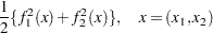
The Levenberg-Marquardt least squares method, which is the method used by the NLPLM subroutine, is a modification of the trust-region method for nonlinear least squares problems. The F_ROSEN module represents the Rosenbrock function. Note that for least squares problems, the  functions
  are specified as elements of a vector; this is different from the manner in which
  is specified for the other optimization techniques. No derivatives are specified in the preceding code, so the NLPLM subroutine computes finite-difference approximations. For more information about the NLPLM subroutine, see the section NLPLM Call.
Constrained Betts Function
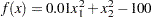
The linearly constrained Betts function (Hock and Schittkowski; 1981) is defined as
 |
The boundary constraints are
 |
 |
 |
|||
 |
 |
|
The linear constraint is
 |
The following code calls the NLPCG subroutine to solve the optimization problem. The infeasible initial point  is specified, and a portion of the output is shown in Figure 14.3.
The NLPCG subroutine performs conjugate gradient optimization. It requires only function and gradient calls. The F_BETTS module represents the Betts function, and since no module is defined to specify the gradient, first-order derivatives are computed by finite-difference approximations. For more information about the NLPCG subroutine, see the section NLPCG Call. For details about the constraint matrix, which is represented by the CON matrix in the preceding code, see the section Parameter Constraints.
| Optimization Start | |||||
|---|---|---|---|---|---|
| Parameter Estimates | |||||
| N | Parameter | Estimate | Gradient Objective Function |
Lower Bound Constraint |
Upper Bound Constraint |
| 1 | X1 | 6.800000 | 0.136000 | 2.000000 | 50.000000 |
| 2 | X2 | -1.000000 | -2.000000 | -50.000000 | 50.000000 |
| Linear Constraints | |||||||||||||
|---|---|---|---|---|---|---|---|---|---|---|---|---|---|
| 1 | 59.00000 | : | 10.0000 | <= | + | 10.0000 | * | X1 | - | 1.0000 | * | X2 | |
| Parameter Estimates | 2 |
|---|---|
| Lower Bounds | 2 |
| Upper Bounds | 2 |
| Linear Constraints | 1 |
| Optimization Start | |||
|---|---|---|---|
| Active Constraints | 0 | Objective Function | -98.5376 |
| Max Abs Gradient Element | 2 | ||
| Iteration | Restarts | Function Calls |
Active Constraints |
Objective Function |
Objective Function Change |
Max Abs Gradient Element |
Step Size |
Slope of Search Direction |
||
|---|---|---|---|---|---|---|---|---|---|---|
| 1 | 0 | 3 | 0 | -99.54682 | 1.0092 | 0.1346 | 0.502 | -4.018 | ||
| 2 | 1 | 7 | 1 | -99.96000 | 0.4132 | 0.00272 | 34.985 | -0.0182 | ||
| 3 | 2 | 9 | 1 | -99.96000 | 1.851E-6 | 0 | 0.500 | -74E-7 |
| Optimization Results | |||
|---|---|---|---|
| Iterations | 3 | Function Calls | 10 |
| Gradient Calls | 9 | Active Constraints | 1 |
| Objective Function | -99.96 | Max Abs Gradient Element | 0 |
| Slope of Search Direction | -7.403546E-6 | ||
| Optimization Results | ||||
|---|---|---|---|---|
| Parameter Estimates | ||||
| N | Parameter | Estimate | Gradient Objective Function |
Active Bound Constraint |
| 1 | X1 | 2.000000 | 0.040000 | Lower BC |
| 2 | X2 | 5.627884E-13 | 0 | |
| Linear Constraints Evaluated at Solution | ||||||||||||
|---|---|---|---|---|---|---|---|---|---|---|---|---|
| 1 | 10.00000 | = | -10.0000 | + | 10.0000 | * | X1 | - | 1.0000 | * | X2 | |
Since the initial point  is infeasible, the subroutine first computes a feasible starting point. Convergence is achieved after three iterations, and the optimal point is given to be
  with an optimal function value of
  . For more information about the printed output, see the section Printing the Optimization History.
Rosen-Suzuki Problem
The Rosen-Suzuki problem is a function of four variables with three nonlinear constraints on the variables. It is taken from problem 43 of Hock and Schittkowski (1981). The objective function is
 |
The nonlinear constraints are
 |
 |
 |
|||
 |
|
 |
|||
|
|
 |
Since this problem has nonlinear constraints, only the NLPQN and NLPNMS subroutines are available to perform the optimization. The following code solves the problem with the NLPQN subroutine:
The F_HS43 module specifies the objective function, and the C_HS43 module specifies the nonlinear constraints. The OPTN vector is passed to the subroutine as the OPT input argument. See the section Options Vector for more information. The value of OPTN[10] represents the total number of nonlinear constraints, and the value of OPTN[11] represents the number of equality constraints. In the preceding code, OPTN[10]=3 and OPTN[11]=0, which indicate that there are three constraints, all of which are inequality constraints. In the subroutine calls, instead of separating missing input arguments with commas, you can specify optional arguments with keywords, as in the CALL NLPQN statement in the preceding code. For details about the CALL NLPQN statement, see the section NLPQN Call.
The initial point for the optimization procedure is  , and the optimal point is
  , with an optimal function value of
  . Part of the output produced is shown in Figure 14.4.
| Optimization Start | ||||
|---|---|---|---|---|
| Parameter Estimates | ||||
| N | Parameter | Estimate | Gradient Objective Function |
Gradient Lagrange Function |
| 1 | X1 | 1.000000 | -3.000000 | -3.000000 |
| 2 | X2 | 1.000000 | -3.000000 | -3.000000 |
| 3 | X3 | 1.000000 | -17.000000 | -17.000000 |
| 4 | X4 | 1.000000 | 9.000000 | 9.000000 |
| Parameter Estimates | 4 |
|---|---|
| Nonlinear Constraints | 3 |
| Optimization Start | |||
|---|---|---|---|
| Objective Function | -19 | Maximum Constraint Violation | 0 |
| Maximum Gradient of the Lagran Func | 17 | ||
| Iteration | Restarts | Function Calls |
Objective Function |
Maximum Constraint Violation |
Predicted Function Reduction |
Step Size |
Maximum Gradient Element of the Lagrange Function |
|
|---|---|---|---|---|---|---|---|---|
| 1 | 0 | 2 | -41.88007 | 1.8988 | 13.6803 | 1.000 | 5.647 | |
| 2 | 0 | 3 | -48.83264 | 3.0280 | 9.5464 | 1.000 | 5.041 | |
| 3 | 0 | 4 | -45.33515 | 0.5452 | 2.6179 | 1.000 | 1.061 | |
| 4 | 0 | 5 | -44.08667 | 0.0427 | 0.1732 | 1.000 | 0.0297 | |
| 5 | 0 | 6 | -44.00011 | 0.000099 | 0.000218 | 1.000 | 0.00906 | |
| 6 | 0 | 7 | -44.00001 | 2.573E-6 | 0.000014 | 1.000 | 0.00219 | |
| 7 | 0 | 8 | -44.00000 | 9.118E-8 | 5.098E-7 | 1.000 | 0.00022 |
| Optimization Results | |||
|---|---|---|---|
| Iterations | 7 | Function Calls | 9 |
| Gradient Calls | 9 | Active Constraints | 2 |
| Objective Function | -44.00000026 | Maximum Constraint Violation | 9.1181918E-8 |
| Maximum Projected Gradient | 0.0002260958 | Value Lagrange Function | -44 |
| Maximum Gradient of the Lagran Func | 0.0002211456 | Slope of Search Direction | -5.098303E-7 |
| Optimization Results | ||||
|---|---|---|---|---|
| Parameter Estimates | ||||
| N | Parameter | Estimate | Gradient Objective Function |
Gradient Lagrange Function |
| 1 | X1 | -0.000001247 | -5.000003 | -0.000012904 |
| 2 | X2 | 1.000027 | -2.999945 | 0.000221 |
| 3 | X3 | 1.999993 | -13.000027 | -0.000053971 |
| 4 | X4 | -1.000003 | 4.999994 | -0.000020534 |
In addition to the standard iteration history, the NLPQN subroutine includes the following information for problems with nonlinear constraints:
CONMAX is the maximum value of all constraint violations.
PRED is the value of the predicted function reduction used with the GTOL and FTOL2 termination criteria.
ALFA is the step size
 of the quasi-Newton step.
 LFGMAX is the maximum element of the gradient of the Lagrange function.