| NLPQN Call |
The NLPQN subroutine uses a quasi-Newton method to compute an optimum value of a function.
See the section Nonlinear Optimization and Related Subroutines for a listing of all NLP subroutines. See Chapter 14 for a description of the arguments of NLP subroutines.
The NLPQN subroutine uses (dual) quasi-Newton optimization techniques, and it is one of the two available subroutines that can solve problems with nonlinear constraints. These techniques work well for medium to moderately large optimization problems where the objective function and the gradient are much faster to compute than the Hessian matrix. The NLPQN subroutine does not need to compute second-order derivatives, but it generally requires more iterations than the techniques that compute second-order derivatives.
The two categories of problems solved by the NLPQN subroutine are unconstrained or linearly constrained problems and nonlinearly constrained problems. Unconstrained or linearly constrained problems do not use the "nlc" or "jacnlc" module arguments, whereas nonlinearly constrained problems use the arguments to specify the nonlinear constraints and the Jacobian matrix of their first-order derivatives, respectively.
The type of optimization problem specified determines the algorithm that the subroutine invokes. The algorithms are very different, and they use different sets of termination criteria. For more details, see the section Termination Criteria.
Unconstrained or Linearly Constrained Quasi-Newton Optimization
The NLPQN subroutine invokes this algorithm if you do not specify the "nlc" argument. Using the fourth element of the opt argument, you can specify two update formulas for either the original quasi-Newton algorithm or the dual quasi-Newton algorithm, as indicated in the following table:
Value of opt[4] |
Update Method |
|---|---|
1 |
Dual Broyden, Fletcher, Goldfarb, and Shanno (DBFGS) update of the Cholesky factor of the Hessian matrix. This is the default. |
2 |
Dual Davidon, Fletcher, and Powell (DDFP) update of the Cholesky factor of the Hessian matrix. |
3 |
Original Broyden, Fletcher, Goldfarb, and Shanno (BFGS) update of the inverse Hessian matrix. |
4 |
Original Davidon, Fletcher, and Powell (DFP) update of the inverse Hessian matrix. |
In each iteration, a line search is performed along the search direction to find an approximate optimum of the objective function. The default line-search method uses quadratic interpolation and cubic extrapolation to obtain a step size that satisfies the Goldstein conditions. One of the Goldstein conditions can be violated if the feasible region defines an upper limit of the step size. Violating the left-side Goldstein condition can affect the positive definiteness of the quasi-Newton update. In these cases, either the update is skipped or the iterations are restarted with an identity matrix that results in the steepest descent or ascent search direction. You can specify line-search algorithms different from the default method with the fifth element of the opt argument.
The following statements invoke the NLPQN subroutine to solve the Rosenbrock problem (see the section Unconstrained Rosenbrock Function):
start F_ROSEN(x);
   y1 = 10 * (x[2] - x[1] * x[1]);
   y2 =  1 - x[1];
   f  = 0.5 * (y1 * y1 + y2 * y2);
   return(f);
finish F_ROSEN;
x = {-1.2 1};
opt = {0 2 . 2};
call nlpqn(rc, xr, "F_ROSEN", x, opt);
Since opt[4]=2, the DDFP update is performed. The gradient is approximated by finite differences since no module is specified that computes the first-order derivatives. Part of the iteration history follows. In addition to the standard iteration history, the NLPQN subroutine prints the following information for unconstrained or linearly constrained problems:
The heading alpha is the step size,
 , computed with the line-search algorithm.
 The heading slope refers to
 , the slope of the search direction at the current parameter iterate
  . For minimization, this value should be significantly smaller than zero. Otherwise, the line-search algorithm has difficulty reducing the function value sufficiently.
| Optimization Start | |||
|---|---|---|---|
| Parameter Estimates | |||
| N | Parameter | Estimate | Gradient Objective Function |
| 1 | X1 | -1.200000 | -107.799989 |
| 2 | X2 | 1.000000 | -43.999999 |
| Parameter Estimates | 2 |
|---|
| Optimization Start | |||
|---|---|---|---|
| Active Constraints | 0 | Objective Function | 12.1 |
| Max Abs Gradient Element | 107.79998927 | ||
| Iteration | Restarts | Function Calls |
Active Constraints |
Objective Function |
Objective Function Change |
Max Abs Gradient Element |
Step Size |
Slope of Search Direction |
||
|---|---|---|---|---|---|---|---|---|---|---|
| 1 | 0 | 4 | 0 | 2.06405 | 10.0359 | 0.7917 | 0.0340 | -628.8 | ||
| 2 | 0 | 7 | 0 | 1.92035 | 0.1437 | 8.6301 | 6.557 | -0.0363 | ||
| 3 | 0 | 10 | 0 | 1.78089 | 0.1395 | 11.0943 | 8.193 | -0.0288 | ||
| 4 | 0 | 13 | 0 | 1.33331 | 0.4476 | 7.6069 | 33.376 | -0.0269 | ||
| 5 | 0 | 17 | 0 | 1.13400 | 0.1993 | 0.9386 | 15.438 | -0.0260 | ||
| 6 | 0 | 22 | 0 | 0.93915 | 0.1948 | 3.5290 | 11.537 | -0.0233 | ||
| 7 | 0 | 24 | 0 | 0.84821 | 0.0909 | 4.8308 | 8.124 | -0.0193 | ||
| 8 | 0 | 30 | 0 | 0.54334 | 0.3049 | 4.1770 | 35.143 | -0.0186 | ||
| 9 | 0 | 32 | 0 | 0.46593 | 0.0774 | 0.9479 | 8.708 | -0.0178 | ||
| 10 | 0 | 37 | 0 | 0.35322 | 0.1127 | 2.5981 | 10.964 | -0.0147 | ||
| 11 | 0 | 40 | 0 | 0.26381 | 0.0894 | 3.3028 | 13.590 | -0.0121 | ||
| 12 | 0 | 41 | 0 | 0.20282 | 0.0610 | 0.6451 | 10.000 | -0.0116 | ||
| 13 | 0 | 46 | 0 | 0.11714 | 0.0857 | 1.6603 | 11.395 | -0.0102 | ||
| 14 | 0 | 51 | 0 | 0.07149 | 0.0456 | 2.4050 | 11.559 | -0.0074 | ||
| 15 | 0 | 53 | 0 | 0.04746 | 0.0240 | 0.5628 | 6.868 | -0.0071 | ||
| 16 | 0 | 58 | 0 | 0.02759 | 0.0199 | 1.3282 | 5.365 | -0.0055 | ||
| 17 | 0 | 60 | 0 | 0.01625 | 0.0113 | 1.9246 | 5.882 | -0.0035 | ||
| 18 | 0 | 62 | 0 | 0.00475 | 0.0115 | 0.6357 | 8.068 | -0.0032 | ||
| 19 | 0 | 66 | 0 | 0.00167 | 0.00307 | 0.4810 | 2.336 | -0.0022 | ||
| 20 | 0 | 70 | 0 | 0.0005952 | 0.00108 | 0.6043 | 3.287 | -0.0006 | ||
| 21 | 0 | 72 | 0 | 0.0000771 | 0.000518 | 0.0289 | 2.329 | -0.0004 | ||
| 22 | 0 | 76 | 0 | 1.92121E-6 | 0.000075 | 0.0365 | 1.772 | -0.0001 | ||
| 23 | 0 | 78 | 0 | 2.39914E-8 | 1.897E-6 | 0.00158 | 1.159 | -331E-8 | ||
| 24 | 0 | 80 | 0 | 5.0936E-11 | 2.394E-8 | 0.000016 | 0.967 | -46E-9 | ||
| 25 | 0 | 119 | 0 | 3.9538E-11 | 1.14E-11 | 7.962E-7 | 1.061 | -19E-13 |
| Optimization Results | |||
|---|---|---|---|
| Iterations | 25 | Function Calls | 120 |
| Gradient Calls | 107 | Active Constraints | 0 |
| Objective Function | 3.953804E-11 | Max Abs Gradient Element | 7.9622469E-7 |
| Slope of Search Direction | -1.88032E-12 | ||
| ABSGCONV convergence criterion satisfied. |
| Optimization Results | |||
|---|---|---|---|
| Parameter Estimates | |||
| N | Parameter | Estimate | Gradient Objective Function |
| 1 | X1 | 0.999991 | -0.000000796 |
| 2 | X2 | 0.999982 | 0.000000430 |
Nonlinearly Constrained Quasi-Newton Optimization
The algorithm used for nonlinearly constrained quasi-Newton optimization is an efficient modification of Powell’s (1978a, 1982b) variable metric constrained watchdog (VMCWD) algorithm. A similar but older algorithm (VF02AD) is part of the Harwell library. Both the VMCWD and VF02AD algorithms use Fletcher’s VE02AD algorithm, which is also part of the Harwell library, for positive definite quadratic programming. This NLPQN implementation uses a quadratic programming subroutine that updates and downdates the Cholesky factor when the active set changes (Gill et al.; 1984). The nonlinear NLPQN algorithm is not a feasible point algorithm, and the value of the objective function is not required to decrease monotonically. Instead, the algorithm tries to reduce a linear combination of objective function and constraint violations.
The following are similarities and differences between this algorithm and Powell’s VMCWD algorithm:
You can use the sixth element of the opt argument to modify the algorithm used by the NLPQN subroutine. If you specify opt[6]
 , which is the default, the evaluation of the Lagrange vector
  is performed the same way as described in Powell (1982). However, the VMCWD program seems to have a bug in the implementation of formula (4.4) in Powell (1982). If you specify opt[6]
 , the original update of used in the VF02AD algorithm in Powell (1978) is performed.
 Instead of updating an approximate Hessian matrix, this algorithm uses the dual BFGS or dual DFP update that updates the Cholesky factor of an approximate Hessian. If the condition of the updated matrix gets too bad, the algorithm restarts with a positive diagonal matrix. At the end of the first iteration after each restart, the Cholesky factor is scaled.
The Cholesky factor is loaded into the quadratic programming subroutine, which ensures positive definiteness of the problem. During the quadratic programming step, the Cholesky factor of the projected Hessian matrix
 is updated simultaneously with
  decomposition when the active set changes. See Gill et al. (1984) for more information.
 The line-search strategy is very similar to that of Powell’s algorithm, but this algorithm does not call for derivatives during the line search. Therefore, this algorithm generally needs fewer derivative calls than function calls, whereas the VMCWD algorithm always requires the same number of derivative calls as function calls. Also, Powell’s line-search method sometimes uses steps that are too long during the early iterations. In those cases, you can use the second element of the par argument to restrict the step length
in the first five iterations. See the section Control Parameters Vector for more details. The watchdog strategy is also similar to that of Powell’s algorithm. However, this algorithm does not return automatically after a fixed number of iterations to a previous, more optimal point. A return to such a point is further delayed if the observed function reduction is close to the expected function reduction of the quadratic model.
Although Powell’s termination criterion, the FTOL2 criterion, can still be used, the NLPQN implementation uses, by default, two other termination criteria (GTOL and ABSGTOL).
This algorithm is automatically invoked if the "nlc" argument is specified. The module specified with the "nlc" argument must return a vector of length  , where is the total number of constraints. Letting
  be the number of equality constraints, the constraints must be of the following form:
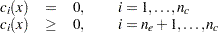 |
The first elements of the returned vector contain the  for the equality constraints, and the remaining elements contain the for the inequality constraints.
Note: You must specify the total number of constraints with the tenth element of the opt argument, and if there are any equality constraints, you must specify their number, , with the eleventh element of the opt argument.
The nonlinear NLPQN algorithm requires the Jacobian matrix of the first-order derivatives of the constraints returned by the module specified by the "nlc" argument. You can provide these derivatives by specifying a module with the "jacnlc" argument. This module must return the Jacobian matrix  of first-order partial derivatives. That is, is an
  matrix such that the entry in the
  th row and
  th column is given by
 |
If you specify an "nlc" module without specifying a "jacnlc" argument, finite difference approximations of the first-order derivatives of the constraints are used. You can use the ninth element of the par argument to specify the number of accurate digits used in evaluating the constraints.
You can specify two update formulas with the fourth element of the opt argument as indicated in the following table:
Value of opt[4] |
Update Method |
|---|---|
1 |
Dual Broyden, Fletcher, Goldfarb, and Shanno (DBFGS) update of the Cholesky factor of the Hessian matrix. This is the default. |
2 |
Dual Davidon, Fletcher, and Powell (DDFP) update of the Cholesky factor of the Hessian matrix. |
This algorithm uses its own line-search technique. None of the options and parameters that control the line search in the other algorithms apply in the nonlinear NLPQN algorithm, with the exception of the second element of the par vector, which can be used to restrict the length of the step size in the first five iterations.
See Example 14.8 for an example where you need to specify a value for the second element of the par argument. The values of the fourth, fifth, and sixth elements of the par vector, which control the processing of linear and boundary constraints, are valid only for the quadratic programming subroutine used in each iteration of the NLPQN call. For a simple example of the NLPQN subroutine, see the section Rosen-Suzuki Problem.