| Time Series Analysis and Examples |
Example 13.4 Diffuse Kalman Filtering
The nonstationary SSM is simulated to analyze the diffuse Kalman filter call KALDFF. The transition equation is generated by using the following formula:
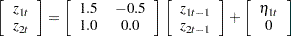 |
where  . The transition equation is nonstationary since the transition matrix
  has one unit root. Here is the code:
proc iml;
z_1 = 0; z_2 = 0;
do i = 1 to 30;
   z = 1.5*z_1 - .5*z_2 + rannor(1234567);
   z_2 = z_1;
   z_1 = z;
   x =  z + .8*rannor(1234578);
   if ( i > 10 ) then y = y // x;
end;
The KALDFF and KALCVF calls produce one-step prediction, and the result shows that two predictions coincide after the fifth observation (Output 13.4.1). Here is the code:
      t = nrow(y);
      h = { 1 0 };
      f = { 1.5 -.5, 1 0 };
      rt = .64;
      vt = diag({1 0});
      ny = nrow(h);
      nz = ncol(h);
      nb = nz;
      nd = nz;
      a  = j(nz,1,0);
      b  = j(ny,1,0);
      int = j(ny+nz,nb,0);
      coef = f // h;
      var = ( vt || j(nz,ny,0) ) //
            ( j(ny,nz,0) || rt );
      intd = j(nz+nb,1,0);
      coefd = i(nz) // j(nb,nd,0);
      at = j(t*nz,nd+1,0);
      mt = j(t*nz,nz,0);
      qt = j(t*(nd+1),nd+1,0);
      n0 = -1;
      call kaldff(kaldff_p,dvpred,initial,s2,y,0,int,
                  coef,var,intd,coefd,n0,at,mt,qt);
      call kalcvf(kalcvf_p,vpred,filt,vfilt,y,0,a,f,b,h,var);
      print kalcvf_p kaldff_p;
| Diffuse Kalman Filtering |
| kalcvf_p | kaldff_p | ||
|---|---|---|---|
| 0 | 0 | 0 | 0 |
| 1.441911 | 0.961274 | 1.1214871 | 0.9612746 |
| -0.882128 | -0.267663 | -0.882138 | -0.267667 |
| -0.723156 | -0.527704 | -0.723158 | -0.527706 |
| 1.2964969 | 0.871659 | 1.2964968 | 0.8716585 |
| -0.035692 | 0.1379633 | -0.035692 | 0.1379633 |
| -2.698135 | -1.967344 | -2.698135 | -1.967344 |
| -5.010039 | -4.158022 | -5.010039 | -4.158022 |
| -9.048134 | -7.719107 | -9.048134 | -7.719107 |
| -8.993153 | -8.508513 | -8.993153 | -8.508513 |
| -11.16619 | -10.44119 | -11.16619 | -10.44119 |
| -10.42932 | -10.34166 | -10.42932 | -10.34166 |
| -8.331091 | -8.822777 | -8.331091 | -8.822777 |
| -9.578258 | -9.450848 | -9.578258 | -9.450848 |
| -6.526855 | -7.241927 | -6.526855 | -7.241927 |
| -5.218651 | -5.813854 | -5.218651 | -5.813854 |
| -5.01855 | -5.291777 | -5.01855 | -5.291777 |
| -6.5699 | -6.284522 | -6.5699 | -6.284522 |
| -4.613301 | -4.995434 | -4.613301 | -4.995434 |
| -5.057926 | -5.09007 | -5.057926 | -5.09007 |
The likelihood function for the diffuse Kalman filter under the finite initial covariance matrix  is written
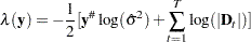 |
where  is the dimension of the matrix
  . The likelihood function for the diffuse Kalman filter under the diffuse initial covariance matrix
  is computed as
 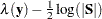 , where the
  matrix is the upper
  matrix of
  . Output 13.4.2 displays the log likelihood and the diffuse log likelihood. Here is the code:
      d = 0;
      do i = 1 to t;
         dt = h*mt[(i-1)*nz+1:i*nz,]*h` + rt;
         d = d + log(det(dt));
      end;
      s = qt[(t-1)*(nd+1)+1:t*(nd+1)-1,1:nd];
      log_l = -(t*log(s2) + d)/2;
      dff_logl = log_l - log(det(s))/2;
      print log_l dff_logl;
Copyright © SAS Institute, Inc. All Rights Reserved.