| Time Series Analysis and Examples |
Example 13.3 Kalman Filtering: SSM Estimation With the EM Algorithm
The following example estimates the normal SSM of the mink-muskrat data by using the EM algorithm. The mink-muskrat series are detrended. Refer to Harvey (1989) for details of this data set. Since this EM algorithm uses filtering and smoothing, you can learn how to use the KALCVF and KALCVS calls to analyze the data. Consider the bivariate SSM:
 |
 |
 |
|||
 |
|
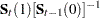
 |
where  is a
is a  identity matrix, the observation noise has a time-invariant covariance matrix
  , and the covariance matrix of the transition equation is also assumed to be time invariant. The initial state
  has mean
  and covariance
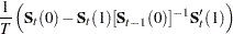
  . For estimation, the matrix is fixed as
 |
while the mean vector is updated by the smoothing procedure such that  . Note that this estimation requires an extra smoothing step since the usual smoothing procedure does not produce
  .
.
The EM algorithm maximizes the expected log-likelihood function given the current parameter estimates. In practice, the log-likelihood function of the normal SSM is evaluated while the parameters are updated by using the M-step of the EM maximization
 |
|
 |
|||
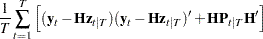
 |
|
 |
|||
 |
|
 |
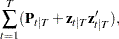
|||
 |
|
 |
where the index  represents the current iteration number, and
 |
|
 |
|||
 |
|
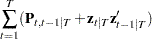 |
It is necessary to compute the value of  recursively such that
 |
where 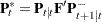 and the initial value
  is derived by using the formula
 |
Note that the initial value of the state vector is updated for each iteration
 |
|
 |
|||
 |
|
 |
The objective function value is computed as  in the IML module LIK. The log-likelihood function is written
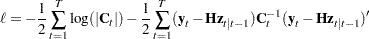 |
where 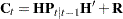 .
.
The iteration history is shown in Output 13.3.1. As shown in Output 13.3.2, the eigenvalues of  are within the unit circle, which indicates that the SSM is stationary. However, the muskrat series (Y1) is reported to be difference stationary. The estimated parameters are almost identical to those of the VAR(1) estimates. Refer to Harvey (1989). Finally, multistep forecasts of
  are computed by using the KALCVF call. Here is the code:
call kalcvf(pred,vpred,filt,vfilt,y,15,a,f,b,h,var,z0,vz0);
The predicted values of the state vector  and their standard errors are shown in Output 13.3.3. Here is the code:
title 'SSM Estimation using EM Algorithm';
data one;
   input y1 y2 @@;
cards;
    0.10609     0.16794
   -0.16852     0.06242
   -0.23700    -0.13344
   -0.18022    -0.50616
    0.18094    -0.37943
    0.65983    -0.40132
    0.65235     0.08789
    0.21594     0.23877
   -0.11515     0.40043
   -0.00067     0.37758
   -0.00387     0.55735
   -0.25202     0.34444
   -0.65011    -0.02749
   -0.53646    -0.41519
   -0.08462     0.02591
   -0.05640    -0.11348
    0.26630     0.20544
    0.03641     0.16331
   -0.26030    -0.01498
   -0.03995     0.09657
    0.33612     0.31096
   -0.11672     0.30681
   -0.69775    -0.69351
   -0.07569    -0.56212
    0.36149    -0.36799
    0.42341    -0.24725
    0.26721     0.04478
   -0.00363     0.21637
    0.08333     0.30188
   -0.22480     0.29493
   -0.13728     0.35463
   -0.12698     0.05490
   -0.18770    -0.52573
    0.34741    -0.49541
    0.54947    -0.26250
    0.57423    -0.21936
    0.57493    -0.12012
    0.28188     0.63556
   -0.58438     0.27067
   -0.50236     0.10386
   -0.60766     0.36748
   -1.04784    -0.33493
   -0.68857    -0.46525
   -0.11450    -0.63648
    0.22005    -0.26335
    0.36533     0.07017
   -0.00151    -0.04977
    0.03740    -0.02411
    0.22438     0.30790
   -0.16196     0.41050
   -0.12862     0.34929
    0.08448    -0.14995
    0.17945    -0.03320
    0.37502     0.02953
    0.95727     0.24090
    0.86188     0.41096
    0.39464     0.24157
    0.53794     0.29385
    0.13054     0.39336
   -0.39138    -0.00323
   -1.23825    -0.56953
   -0.66286    -0.72363
;
proc iml;
   start lik(y,pred,vpred,h,rt);
       n = nrow(y);
       nz = ncol(h);
       et = y - pred*h`;
       sum1 = 0;
       sum2 = 0;
       do i = 1 to n;
          vpred_i = vpred[(i-1)*nz+1:i*nz,];
          et_i = et[i,];
          ft = h*vpred_i*h` + rt;
          sum1 = sum1 + log(det(ft));
          sum2 = sum2 + et_i*inv(ft)*et_i`;
       end;
       return(sum1+sum2);
   finish;

   start main;
      use one;
      read all into y var {y1 y2};
     /*-- mean adjust series --*/
      t = nrow(y);
      ny = ncol(y);
      nz = ny;
      f = i(nz);
      h = i(ny);

      /*-- observation noise variance is diagonal --*/
      rt = 1e-5#i(ny);

      /*-- transition noise variance --*/
      vt = .1#i(nz);
      a = j(nz,1,0);
      b = j(ny,1,0);
      myu = j(nz,1,0);
      sigma = .1#i(nz);
      converge = 0;
      logl0 = 0.0;
      do iter = 1 to 100 while( converge = 0 );


      /*--- construct big cov matrix --*/
      var = ( vt || j(nz,ny,0) ) //
            ( j(ny,nz,0) || rt );

      /*-- initial values are changed --*/
      z0  = myu` * f`;
      vz0 = f * sigma * f` + vt;

      /*-- filtering to get one-step prediction and filtered value --*/
      call kalcvf(pred,vpred,filt,vfilt,y,0,a,f,b,h,var,z0,vz0);

      /*-- smoothing using one-step prediction values --*/
      call kalcvs(sm,vsm,y,a,f,b,h,var,pred,vpred);

      /*-- compute likelihood values --*/
      logl = lik(y,pred,vpred,h,rt);

      /*-- store old parameters and function values --*/
      myu0 = myu;
      f0 = f;
      vt0 = vt;
      rt0 = rt;
      diflog = logl - logl0;
      logl0 = logl;
      itermat = itermat // ( iter || logl0 || shape(f0,1) || myu0` );

      /*-- obtain P*(t) to get P_T_0 and Z_T_0   --*/
      /*-- these values are not usually needed   --*/
      /*-- See Harvey (1989 p154) or Shumway (1988, p177) --*/
      jt1 = sigma * f` * inv(vpred[1:nz,]);
      p_t_0  = sigma + jt1*(vsm[1:nz,] - vpred[1:nz,])*jt1`;
      z_t_0  = myu + jt1*(sm[1,]` - pred[1,]`);
      p_t1_t  = vpred[(t-1)*nz+1:t*nz,];
      p_t1_t1 = vfilt[(t-2)*nz+1:(t-1)*nz,];
      kt = p_t1_t*h`*inv(h*p_t1_t*h`+rt);

      /*-- obtain P_T_TT1. See Shumway (1988, p180) --*/
      p_t_ii1 = (i(nz)-kt*h)*f*p_t1_t1;
      st0 = vsm[(t-1)*nz+1:t*nz,] + sm[t,]`*sm[t,];
      st1 = p_t_ii1 + sm[t,]`*sm[t-1,];
      st00 = p_t_0 + z_t_0 * z_t_0`;
      cov = (y[t,]` - h*sm[t,]`) * (y[t,]` - h*sm[t,]`)` +
            h*vsm[(t-1)*nz+1:t*nz,]*h`;
      do i = t to 2 by -1;
         p_i1_i1 = vfilt[(i-2)*nz+1:(i-1)*nz,];
         p_i1_i  = vpred[(i-1)*nz+1:i*nz,];
         jt1 = p_i1_i1 * f` * inv(p_i1_i);
         p_i1_i  = vpred[(i-2)*nz+1:(i-1)*nz,];
         if ( i > 2 ) then
            p_i2_i2 = vfilt[(i-3)*nz+1:(i-2)*nz,];
         else
            p_i2_i2 = sigma;
         jt2 = p_i2_i2 * f` * inv(p_i1_i);
         p_t_i1i2 = p_i1_i1*jt2` + jt1*(p_t_ii1 - f*p_i1_i1)*jt2`;
         p_t_ii1 = p_t_i1i2;
         temp = vsm[(i-2)*nz+1:(i-1)*nz,];
         sm1 = sm[i-1,]`;
         st0 = st0 + ( temp + sm1 * sm1` );
         if ( i > 2 ) then
            st1 = st1 + ( p_t_ii1 + sm1 * sm[i-2,]);
         else st1 = st1 + ( p_t_ii1 + sm1 * z_t_0`);
         st00 = st00 + ( temp + sm1 * sm1` );
         cov = cov + ( h * temp * h` +
               (y[i-1,]` - h * sm1)*(y[i-1,]` - h * sm1)` );
      end;

      /*-- M-step: update the parameters --*/
      myu = z_t_0;
      f = st1 * inv(st00);
      vt = (st0 - st1 * inv(st00) * st1`)/t;
      rt = cov / t;

      /*-- check convergence --*/
      if ( max(abs((myu - myu0)/(myu0+1e-6))) < 1e-2 &
           max(abs((f - f0)/(f0+1e-6))) < 1e-2 &
           max(abs((vt - vt0)/(vt0+1e-6))) < 1e-2 &
           max(abs((rt - rt0)/(rt0+1e-6))) < 1e-2 &
           abs((diflog)/(logl0+1e-6)) < 1e-3 ) then
         converge = 1;
      end;


      reset noname;
         colnm = {'Iter' '-2*log L' 'F11' 'F12' 'F21' 'F22'
               'MYU11' 'MYU22'};
      print itermat[colname=colnm format=8.4];

      eval = eigval(f0);
      colnm = {'Real' 'Imag' 'MOD'};
      eval = eval || sqrt((eval#eval)[,+]);
      print eval[colname=colnm];
      var = ( vt || j(nz,ny,0) ) //
            ( j(ny,nz,0) || rt );

      /*-- initial values are changed --*/
      z0  = myu` * f`;
      vz0 = f * sigma * f` + vt;
      free itermat;

      /*-- multistep prediction --*/
      call kalcvf(pred,vpred,filt,vfilt,y,15,a,f,b,h,var,z0,vz0);
      do i = 1 to 15;
         itermat = itermat // ( i || pred[t+i,] ||
                   sqrt(vecdiag(vpred[(t+i-1)*nz+1:(t+i)*nz,]))` );
      end;
      colnm = {'n-Step' 'Z1_T_n' 'Z2_T_n' 'SE_Z1' 'SE_Z2'};
      print itermat[colname=colnm];
   finish;
   run;
| SSM Estimation using EM Algorithm |
| Iter | -2*log L | F11 | F12 | F21 | F22 | MYU11 | MYU22 |
|---|---|---|---|---|---|---|---|
| 1.0000 | -154.010 | 1.0000 | 0.0000 | 0.0000 | 1.0000 | 0.0000 | 0.0000 |
| 2.0000 | -237.962 | 0.7952 | -0.6473 | 0.3263 | 0.5143 | 0.0530 | 0.0840 |
| 3.0000 | -238.083 | 0.7967 | -0.6514 | 0.3259 | 0.5142 | 0.1372 | 0.0977 |
| 4.0000 | -238.126 | 0.7966 | -0.6517 | 0.3259 | 0.5139 | 0.1853 | 0.1159 |
| 5.0000 | -238.143 | 0.7964 | -0.6519 | 0.3257 | 0.5138 | 0.2143 | 0.1304 |
| 6.0000 | -238.151 | 0.7963 | -0.6520 | 0.3255 | 0.5136 | 0.2324 | 0.1405 |
| 7.0000 | -238.153 | 0.7962 | -0.6520 | 0.3254 | 0.5135 | 0.2438 | 0.1473 |
| 8.0000 | -238.155 | 0.7962 | -0.6521 | 0.3253 | 0.5135 | 0.2511 | 0.1518 |
| 9.0000 | -238.155 | 0.7962 | -0.6521 | 0.3253 | 0.5134 | 0.2558 | 0.1546 |
| 10.0000 | -238.155 | 0.7961 | -0.6521 | 0.3253 | 0.5134 | 0.2588 | 0.1565 |
| n-Step | Z1_T_n | Z2_T_n | SE_Z1 | SE_Z2 |
|---|---|---|---|---|
| 1 | -0.055792 | -0.587049 | 0.2437666 | 0.237074 |
| 2 | 0.3384325 | -0.319505 | 0.3140478 | 0.290662 |
| 3 | 0.4778022 | -0.053949 | 0.3669731 | 0.3104052 |
| 4 | 0.4155731 | 0.1276996 | 0.4021048 | 0.3218256 |
| 5 | 0.2475671 | 0.2007098 | 0.419699 | 0.3319293 |
| 6 | 0.0661993 | 0.1835492 | 0.4268943 | 0.3396153 |
| 7 | -0.067001 | 0.1157541 | 0.430752 | 0.3438409 |
| 8 | -0.128831 | 0.0376316 | 0.4341532 | 0.3456312 |
| 9 | -0.127107 | -0.022581 | 0.4369411 | 0.3465325 |
| 10 | -0.086466 | -0.052931 | 0.4385978 | 0.3473038 |
| 11 | -0.034319 | -0.055293 | 0.4393282 | 0.3479612 |
| 12 | 0.0087379 | -0.039546 | 0.4396666 | 0.3483717 |
| 13 | 0.0327466 | -0.017459 | 0.439936 | 0.3485586 |
| 14 | 0.0374564 | 0.0016876 | 0.4401753 | 0.3486415 |
| 15 | 0.0287193 | 0.0130482 | 0.440335 | 0.3487034 |
Copyright © SAS Institute, Inc. All Rights Reserved.