The QR subroutine produces the QR decomposition of a matrix by using Householder transformations.

The QR subroutine returns the following values:

q

specifies an orthogonal matrix that is the product of the Householder transformations applied to the matrix , if the argument is not specified. In this case, the Householder transformations are applied, and is an matrix. If the argument is specified, is the matrix that has the transposed Householder transformations applied on the columns of the argument matrix .

r

specifies a upper triangular matrix that is the upper part of the upper triangular matrix of the QR decomposition of the matrix . The matrix of the QR decomposition can be obtained by vertical concatenation (by using the operator //) of the zero matrix to the result matrix .

piv

specifies an vector of permutations of the columns of ; that is, on return, the QR decomposition is computed, not of , but of the permuted matrix whose columns are . The vector piv corresponds to an permutation matrix .

lindep

is the number of linearly dependent columns in matrix detected by applying the Householder transformations in the order specified by the argument vector piv.

The input arguments to the QR subroutine are as follows:

a

specifies an matrix that is to be decomposed into the product of the orthogonal matrix and the upper triangular matrix .

ord

specifies an optional vector that specifies the order of Householder transformations applied to matrix , as follows:

ord[j]>0

Column of is an initial column, meaning it has to be processed at the start in increasing order of ord[j].

ord[j]=0

Column of can be permuted in order of decreasing residual Euclidean norm (pivoting).

ord[j]<0

Column of is a final column, meaning it has to be processed at the end in decreasing order of ord[j].

The default is ord[j]=j, in which case the Householder transformations are done in the same order that the columns are stored in matrix (without pivoting).

b

specifies an optional matrix that is to be multiplied by the transposed matrix . If is specified, the result contains the matrix . If is not specified, the result contains the matrix .

The QR subroutine decomposes an matrix into the product of an orthogonal matrix and an upper triangular matrix , so that

by means of Householder transformations.

The orthogonal matrix is computed only if the last argument is not specified, as in the following example:

   call qr(q,r,piv,lindep,a,ord);

In many applications, the number of rows, , is very large. In these cases, the explicit computation of the matrix can require too much memory or time.

In the usual case where ,

where is the result returned by the QR subroutine.

The columns of matrix provide an orthonormal basis for the columns of and are called the range space of . Since the columns of are orthogonal to the columns of , , they provide an orthonormal basis for the orthogonal complement of the columns of and are called the null space of .

In the case where ,

Specifying the argument ord as an vector lets you specify a special order of the columns in matrix on which the Householder transformations are applied. When you specify the ord argument, the columns of can be divided into the following groups:

• ord[j]>0: Column of is an initial column, meaning it has to be processed at the start in increasing order of ord[j]. This specification defines the first columns of that are to be processed.

• ord[j]=0: Column of is a pivot column, meaning it is to be processed in order of decreasing residual Euclidean norms. The pivot columns of are processed after the initial columns and before the final columns.

• ord[j]<0: Column of is a final column, meaning it has to be processed at the end in decreasing order of ord. This specification defines the last columns of that are to be processed. If , some of these columns will not be processed at all.

There are two special cases:

• If you do not specify the ord argument, the default values ord are used. In this case, Householder transformations are done in the same order in which the columns are stored in (without pivoting).

• If you set all components of ord to zero, the Householder transformations are done in order of decreasing Euclidean norms of the columns of .

The resulting vector piv specifies the permutation of the columns of on which the Householder transformations are applied; that is, on return, the QR decomposition is computed, not of , but of the matrix with columns that are permuted in the order .

To check the QR decomposition, use the following statements to compute the three residual sum of squares, represented by the variables SS0, SS1, and SS2, which should be close to zero:

   m = nrow(a); n = ncol(a);
   call qr(q,r,piv,lindep,a,ord);
   ss0 = ssq(a[ ,piv] - q[,1:n] * r);
   ss1 = ssq(q * q` - i(m));
   ss2 = ssq(q` * q - i(m));

If the QR subroutine detects linearly dependent columns while processing matrix , the column order given in the result vector piv can differ from an explicitly specified order in the argument vector ord. If a column of is found to be linearly dependent on columns already processed, this column is swapped to the end of matrix . The order of columns in the result matrix corresponds to the order of columns processed in . The swapping of a linearly dependent column of to the end of the matrix corresponds to the swapping of the same column in and leads to a zero row at the end of the upper triangular matrix .

The scalar result lindep counts the number of linearly dependent columns that are detected in constructing the first Householder transformations in the order specified by the argument vector ord. The test of linear dependence depends on the size of the singularity criterion used; currently it is specified as 1E8.

Solving the linear system with an upper triangular matrix whose columns are permuted corresponding to the result vector piv leads to a solution with permuted components. You can reorder the components of by using the index vector piv at the left-hand side of an expression, as follows:

   call qr(qtb,r,piv,lindep,a,ord,b);
   x[piv] = inv(r) * qtb[1:n,1:p];

The following example solves the full-rank linear least squares problem. Specify the argument as an matrix , as follows:

   call qr(q,r,piv,lindep,a,ord,b);

When you specify the argument, the QR call computes the matrix (instead of ) as the result . Now you can compute the least squares solutions of an overdetermined linear system with an coefficient matrix , rank() = , and right-hand sides stored as the columns of the matrix :

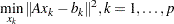where is the Euclidean vector norm. This is accomplished by solving the upper triangular systems with back-substitution:

For most applications, , the number of rows of , is much larger than , the number of columns of , or , the number of right-hand sides. In these cases, you are advised not to compute the large matrix (which can consume too much memory and time) if you can solve your problem by computing only the smaller matrix implicitly. For example, use the first five columns of the Hilbert matrix , as follows:

   a= {  36      -630      3360     -7560      7560     -2772,
       -630     14700    -88200    211680   -220500     83160,
       3360    -88200    564480  -1411200   1512000   -582120,
      -7560    211680  -1411200   3628800  -3969000   1552320,
       7560   -220500   1512000  -3969000   4410000  -1746360,
      -2772     83160   -582120   1552320  -1746360    698544 };
   b= { 463, -13860, 97020, -258720, 291060, -116424};
   n = 5; aa = a[,1:n];
   call qr(qtb,r,piv,lindep,aa,,b);
   if lindep=0 then x=inv(r)*qtb[1:n];
   print x;

Note that you are using only the first rows, , of QTB. The IF-THEN statement of the preceding example can be replaced by the more efficient TRISOLV function, as follows:

   if lindep=0 then x=trisolv(1,r,qtb[1:n],piv);
   print x;

Both cases produce the following output:

            X
            1
          0.5
    0.3333333
         0.25
          0.2

For information about solving rank-deficient linear least squares problems, see the RZLIND call.