The QUAD subroutine performs numerical integration of scalar functions in one dimension over infinite, connected semi-infinite, and connected finite intervals.

The QUAD subroutine returns the following value:

r

is a numeric vector that contains the results of the integration. The size of is equal to the number of subintervals defined by the argument points. Should the numerical integration fail on a particular subinterval, the corresponding element of is set to missing.

The input arguments to the QUAD subroutine are as follows:

"fun"

specifies the name of a module used to evaluate the integrand.

points

specifies a sorted vector that provides the limits of integration over connected subintervals. The simplest form of the vector provides the limits of the integration on one interval. The first element of points should contain the left limit. The second element should be the right limit. A missing value of .M in the left limit is interpreted as , and a missing value of .P is interpreted as . For more advanced usage of the QUAD call, points can contain more than two elements. The elements of the vector must be sorted in an ascending order. Each two consecutive elements in points defines a subinterval, and the subroutine reports the integration over each specified subinterval. The use of subintervals is important because the presence of internal points of discontinuity in the integrand hinders the algorithm.

eps

is an optional scalar that specifies the desired relative accuracy. It has a default value of 1E7. You can specify eps with the keyword EPS.

peak

is an optional scalar that is the approximate location of a maximum of the integrand. By default, it has a location of 0 for infinite intervals, a location that is one unit away from the finite boundary for semi-infinite intervals, and a centered location for bounded intervals. You can specify peak with the keyword PEAK.

scale

is an optional scalar that is the approximate estimate of any scale in the integrand along the independent variable (see the examples). It has a default value of 1. You can specify scale with the keyword SCALE.

msg

is an optional character scalar that restricts the number of messages produced by the QUAD subroutine. If msg = "NO" then it does not produce any warning messages. You can specify msg with the keyword MSG.

cycles

is an optional integer that indicates the maximum number of refinements the QUAD subroutine can make in order to achieve the required accuracy. It has a default value of 8. You can specify cycles with the keyword CYCLES.

If the dimensions of any optional argument are , the QUAD subroutine uses its default value.

The QUAD subroutine is a numerical integrator based on adaptive Romberg-type integration techniques. see Rice (1973), Sikorsky (1982), Sikorsky and Stenger (1984), Stenger (1973a), Stenger (1973b), and Stenger (1978). Many adaptive numerical integration methods (Ralston and Rabinowitz; 1978) start at one end of the interval and proceed towards the other end, working on subintervals while locally maintaining a certain prescribed precision. This is not the case with the QUAD call. The QUAD call is an adaptive global-type integrator that produces a quick, rough estimate of the integration result and then refines the estimate until achieving the prescribed accuracy. This gives the subroutine an advantage over Gauss-Hermite and Gauss-Laguerre quadratures (Ralston and Rabinowitz; 1978), (Squire; 1987), particularly for infinite and semi-infinite intervals, because those methods perform only a single evaluation.

Consider the integral

The following statements evaluate this integral:

  /* Define the integrand */
  start fun(t);
      v = exp(-t);
      return(v);
  finish;

  /* Call QUAD */
  a   = { 0  .P };
  call quad(z,"fun",a);
  print z[format=E21.14];

The integration is carried out over the interval , as specified by the variable A. Note that the missing value in the second element of A is interpreted as . The values of eps=1E7, peak=1, scale=1, and cycles=8 are used by default.

The following statements perform the integration over two subintervals, as specified by the variable A:

  /* Define the integrand */
  start fun(t);
      v = exp(-t);
      return(v);
  finish;

  /* Call QUAD */
  a   = { 0  3 .P };
  call quad(z,"fun",a);
  print z[format=E21.14];

Note that the elements of A are in ascending order. The integration is carried out over and , and the corresponding results are shown in the output. The values of eps=1E7, peak=1, scale=1, and cycles=8 are used by default. To obtain the results of integration over , use the SUM function on the elements of the vector , as follows:

    b = sum(z);
    print b[format=E21.14];

The purpose of the peak and scale options is to enable you to avoid analytically changing the variable of the integration in order to produce a well-conditioned integrand that permits the numerical evaluation of the integration.

Consider the integration

The following statements evaluate this integral:

  /* Define the integrand */
  start fun(t);
      v = exp(-10000*t);
      return(v);
  finish;

  /* Call QUAD */
  a   = { 0  .P };
  /* Either syntax can be used               */
  /*   call quad(z,"fun",a,1E-10,0.0001); or */
  call quad(z,"fun",a) eps=1E-10 peak=0.0001 ;
  print z[format=E21.14];

Only one interval exists. The integration is carried out over . The default values of scale=1 and cycles=8 are used.

If you do not specify a peak value, the integration cannot be evaluated to the desired accuracy, a message is printed to the LOG, and a missing value is returned. Note that peak can still be set to 1E7 and the integration will be successful. The evaluation of the integrand at peak must be nonzero for the computation to continue. You should adjust the value of peak to get a nonzero evaluation at peak before trying to adjust scale. Reducing scale decreases the initial step size and can lead to an increase in the number of function evaluations per step at a linear rate.

Consider the integration

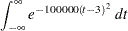The following statements evaluate this integral:

  /* Define the integrand */
  start fun(t);
      v = exp(-100000*(t-3)*(t-3));
      return(v);
  finish;
  /* Call QUAD */
  a   = { .M  .P };
  call quad(z,"fun",a) eps=1E-10 peak=3 scale=0.001 ;
  print z[format=E21.14];

Only one interval exists. The integration is carried out over . The default value of cycles=8 has been used.

If you use the default value of scale, the integral cannot be evaluated to the desired accuracy, and a missing value is returned. The variables scale and cycles can be used to increase the number of possible function evaluations; the number of possible function evaluations increases linearly with the reciprocal of scale, but it potentially increases in an exponential manner when cycles is increased. Increasing the number of function evaluations increases execution time.

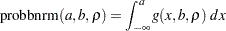
When you perform double integration, you must separate the variables between the iterated integrals. There should be a clear distinction between the variables of the one-dimensional integration at hand and the parameters to be passed to the integrand. Posting the correct limits of integration is also an important issue. For example, consider the binormal probability, given by

The inner integral is

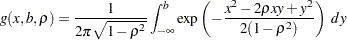with parameters and , and the limits of integration are from to . The outer integral is then

with the limits from to .

You can write the equation in the form of a function with the parameters as arguments. The following statements provide an example of this technique:

   start norpdf2(t) global(yv,rho,omrho2,count);

   /*-----------------------------------------------------*/
   /* This function is the density function and requires  */
   /* the variable T (passed in the argument)             */
   /* and a list of parameters, YV, RHO, OMRHO2, COUNT    */
   /* (defined in the GLOBAL clause)                      */
   /*-----------------------------------------------------*/

      count = count+1;
      q=(t#t-2#rho#t#yv+yv#yv)/omrho2;
      p=exp(-q/2);
      return(p);
   finish;

   start marginal(v) global(yy,yv,eps);
   /*--------------------------------------------------*/
   /* The inner integral                               */
   /* The limits of integration from .M to YY          */
   /* YV is passed as a parameter to the inner integral*/
   /*--------------------------------------------------*/
      interval = .M || yy;
      if ( v < -12 ) then return(0);
      yv = v;
      call quad(pm,"NORPDF2",interval) eps=eps;
      return(pm);
   finish;

   start norcdf2(a,b,rrho) global(yy,rho,omrho2,eps);
   /*------------------------------------------------*/
   /* Post some global parameters                    */
   /*    YY, RHO, OMRHO2                             */
   /* EPS will be set from IML                       */
   /* RHO and B cannot be arguments in the GLOBAL    */
   /* list at the same time                          */
   /*------------------------------------------------*/
      rho = rrho;
      yy = b;
      omrho2 = 1-rho#rho;
      /*----------------------------------------------*/
      /* The outer integral                           */
      /* The limits of integration                    */
      /*----------------------------------------------*/
      interval= .M || a;

      /*----------------------------------------------*/
      /*Note that EPS the keyword = EPS the variable  */
      /*----------------------------------------------*/
      call quad(p,"MARGINAL",interval) eps=eps;

      /*--------------------------*/
      /*  PER will be reset here  */
      /*--------------------------*/
      per = 1/(8#atan(1)#sqrt(omrho2)) * p;
      return(per);
   finish;

   /*----------------------------------*/
   /*First set up the global constants */
   /*----------------------------------*/
   count = 0;
   eps = 1E-11;

   /*------------------------------------*/
   /* Do the work and print the results  */
   /*------------------------------------*/
   p =  norcdf2(2,1,0.1);
   print p[format=E21.14];
   print count;

The variable COUNT contains the number of times the NORPDF2 module is called. Note that the value computed by the NORCDF2 module is very close to that returned by the PROBBNRM function, as computed by the following statements:

   /*------------------------------------------------*/
   /* Compute the value with the PROBBNRM function */
   /*------------------------------------------------*/
   pp = probbnrm(2,1,0.1);
   print pp[format=E21.14];

Note the following:

• The iterated inner integral cannot have a left endpoint of . For large values of , the inner integral does not contribute to the answer but still needs to be computed to the required relative accuracy. Therefore, either cut off the function (when ), as in the MARGINAL module in the preceding example, or have the intervals start from a reasonable cutoff value. In addition, the QUAD call stops if the integrands appear to be identically 0 (probably caused by underflow) over the interval of integration.

• This method of integration (iterated, one-dimensional integrals) is extremely conservative and requires unnecessary function evaluations. In this example, the QUAD call for the inner integration lacks information about the final value that the QUAD call for the outer integration is trying to refine. The lack of communication between the two QUAD routines can cause useless computations to be performed in the inner integration.

  To illustrate this idea, let the relative error be 1E11 and let the answer delivered by the outer integral be 0.8, as in this example. Any computation of the inner execution of the QUAD call that yields 0.8E11 or less does not contribute to the final answer of the QUAD call for the outer integral. However, the inner integral lacks this information, and for a given value of the parameter , it attempts to compute an answer with much more precision than is necessary. The lack of communication between the two QUAD subroutines prevents the introduction of better cut-offs. Although this method can be inefficient, the final calculations are accurate.