The RZLIND subroutine computes rank-deficient linear least squares solutions, complete orthogonal factorizations, and Moore-Penrose inverses.

The RZLIND subroutine returns the following values:

lindep

is a scalar that contains the number of linear dependencies that are recognized in (number of zeroed rows in rup[n,n]).

rup

is the updated upper triangular matrix that contains zero rows corresponding to zero recognized diagonal elements in the original .

bup

is the matrix of right-hand sides that is updated simultaneously with . If is not specified, bup is not accessible.

The input arguments to the RZLIND subroutine are as follows:

r

specifies the upper triangular matrix . Only the upper triangle of is used; the lower triangle can contain any information.

sing

is an optional scalar that specifies a relative singularity criterion for the diagonal elements of . The diagonal element is considered zero if
, where is the Euclidean norm of column of . If the value provided for sing is not positive, the default value sing is used, where is the relative machine precision.

b

specifies the optional matrix of right-hand sides that have to be updated or downdated simultaneously with .

The singularity test used in the RZLIND subroutine is a relative test that uses the Euclidean norms of the columns of . The diagonal element is considered as nearly zero (and the th row is zeroed out) if the following test is true:

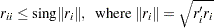Providing an argument sing is the same as omitting the argument sing in the RZLIND call. In this case, the default is sing, where is the relative machine precision. If is computed by the QR decomposition , then the Euclidean norm of column of is the same (except for rounding errors) as the Euclidean norm of column of .

Consider the following possible application of the RZLIND subroutine. Assume that you want to compute the upper triangular Cholesky factor of the positive semidefinite matrix ,

The Cholesky factor of a positive definite matrix is unique (with the exception of the sign of its rows). However, the Cholesky factor of a positive semidefinite (singular) matrix can have many different forms.

In the following example, is a matrix with linearly dependent columns and with , , and .

   a = {1 1 0 0 1 0 0,
        1 1 0 0 1 0 0,
        1 1 0 0 0 1 0,
        1 1 0 0 0 0 1,
        1 0 1 0 1 0 0,
        1 0 1 0 0 1 0,
        1 0 1 0 0 1 0,
        1 0 1 0 0 0 1,
        1 0 0 1 1 0 0,
        1 0 0 1 0 1 0,
        1 0 0 1 0 0 1,
        1 0 0 1 0 0 1};
   a = a || uniform(j(12,1,1));
   aa = a` * a;
   m = nrow(a); n = ncol(a);

Applying the ROOT function to the coefficient matrix of the normal equations generates an upper triangular matrix where linearly dependent rows are zeroed out. You can verify that . Here is the code:

   r1 = root(aa);
   ss1 = ssq(aa - r1` * r1);
   print ss1 r1 [format=best6.];

Applying the QR subroutine with column pivoting on the original matrix yields a different result, but you can also verify after pivoting the rows and columns of . Here is the code:

   ord = j(n,1,0);
   call qr(q,r2,pivqr,lindqr,a,ord);
   ss2 = ssq(aa[pivqr,pivqr] - r2` * r2);
   print ss2 r2 [format=best6.];

Using the RUPDT subroutine for stepwise updating of by the rows of finally results in an upper triangular matrix with nearly zero diagonal elements. However, other elements in rows with nearly zero diagonal elements can have significant values. The following statements verify that :

   r3 = shape(0,n,n);
   call rupdt(rup,bup,sup,r3,a);
   r3 = rup;
   ss3 = ssq(aa - r3` * r3);
   print ss3 r3 [format=best6.];

The result of the RUPDT subroutine can be transformed into the result of the ROOT function by left applications of Givens rotations to zero out the remaining significant elements of rows with small diagonal elements. Applying the RZLIND subroutine on the upper triangular result of the RUPDT subroutine generates a Cholesky factor with zero rows corresponding to diagonal elements that are small, giving the same result as the ROOT function (except for the sign of rows) if its singularity criterion recognizes the same linear dependencies. Here is the code:

   call rzlind(lind,r4,bup,r3);
   ss4 = ssq(aa - r4` * r4);
   print ss4 r4 [format=best6.];

Consider the rank-deficient linear least squares problem:

For , the optimal solution, , is unique; however, for , the rank-deficient linear least squares problem has many optimal solutions, each of which has the same least squares residual sum of squares:

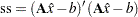The solution of the full-rank problem, , is illustrated in the QR call. The following list shows several solutions to the singular problem. The following example uses the matrix from the preceding section and generates a new column vector . The vector and the matrix are shown in the output.

   b = uniform(j(12,1,1));
   ab = a` * b;
   print b a [format=best6.];

Each entry in the following list solves the rank-deficient linear least squares problem. Note that while each method minimizes the residual sum of squares, not all of the given solutions are of minimum Euclidean length.

• Use the singular value decomposition of , given by . Take the reciprocals of significant singular values and set the small values of to zero.

           call svd(u,d,v,a);
           t = 1e-12 * d[1];
           do i=1 to n;
              if d[i] < t then d[i] = 0.;
              else d[i] = 1. / d[i];
           end;
           x1 = v * diag(d) * u` * b;
           len1 = x1` * x1;
           ss1 = ssq(a * x1 - b);
           x1 = x1`;
           print ss1 len1, x1 [format=best6.];
        

  The solution obtained by singular value decomposition, , is of minimum Euclidean length.

• Use QR decomposition with column pivoting:

  Set the right part to zero and invert the upper triangular matrix to obtain a generalized inverse and an optimal solution :

           ord = j(n,1,0);
           call qr(qtb,r2,pivqr,lindqr,a,ord,b);
           nr = n - lindqr;
           r = r2[1:nr,1:nr];
           x2 = shape(0,n,1);
           x2[pivqr] = trisolv(1,r,qtb[1:nr]) // j(lindqr,1,0.);
           len2 = x2` * x2;
           ss2 = ssq(a * x2 - b);
           x2 = x2`;
           print ss2 len2, x2 [format=best6.];
        

  Note that the residual sum of squares is minimal, but the solution is not of minimum Euclidean length.

• Use the result of the ROOT function on to obtain the vector piv which indicates the zero rows in the upper triangular matrix :

           r1 = root(aa);
           nr = n - lind;
           piv = shape(0,n,1);
           j1 = 1; j2 = nr + 1;
           do i=1 to n;
              if r1[i,i] ^= 0 then do;
                 piv[j1] = i; j1 = j1 + 1;
              end;
              else do;
                 piv[j2] = i; j2 = j2 + 1;
              end;
           end;
        

  Now compute by solving the equation .

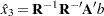           r  = r1[piv[1:nr],piv[1:nr]];
           x  = trisolv(2,r,ab[piv[1:nr]]);
           x  = trisolv(1,r,x);
           x3 = shape(0,n,1);
           x3[piv] = x // j(lind,1,0.);
           len3 = x3` * x3;
           ss3  = ssq(a * x3 - b);
           x3 = x3`;
           print ss3 len3, x3 [format=best6.];
        

  Note that the residual sum of squares is minimal, but the solution is not of minimum Euclidean length.

• Use the result of the RUPDT call on and the vector piv (obtained in the previous solution), which indicates the zero rows of upper triangular matrices and . After zeroing out the rows of belonging to small diagonal pivots, solve the system .

           r3 = shape(0,n,n);
           qtb = shape(0,n,1);
           call rupdt(rup,bup,sup,r3,a,qtb,b);
           r3 = rup; qtb = bup;
           call rzlind(lind,r4,bup,r3,,qtb);
           qtb = bup[piv[1:nr]];
           x  = trisolv(1,r4[piv[1:nr],piv[1:nr]],qtb);
           x4 = shape(0,n,1);
           x4[piv] = x // j(lind,1,0.);
           len4 = x4` * x4;
           ss4 = ssq(a * x4 - b);
           x4 = x4`;
           print ss4 len4, x4 [format=best6.];
        

  Since the matrices and are the same (except for the signs of rows), the solution is the same as .

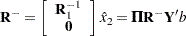
• Use the result of the RZLIND call in the previous solution, which is the result of the first step of complete QR decomposition, and perform the second step of complete QR decomposition. The rows of matrix can be permuted to the upper trapezoidal form

  where is nonsingular and upper triangular and is rectangular. Next, perform the second step of complete QR decomposition with the lower triangular matrix

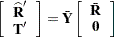
  which leads to the upper triangular matrix .

           r = r4[piv[1:nr],]`;
           call qr(q,r5,piv2,lin2,r);
           y  = trisolv(2,r5,qtb);
           x5 = q * (y // j(lind,1,0.));
           len5 = x5` * x5;
           ss5 = ssq(a * x5 - b);
           x5 = x5`;
           print ss5 len5, x5 [format=best6.];
        

  The solution obtained by complete QR decomposition has minimum Euclidean length.

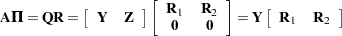
• Perform both steps of complete QR decomposition. The first step performs the pivoted QR decomposition of ,

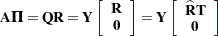
  where is nonsingular and upper triangular and is rectangular. The second step performs a QR decomposition as described in the previous method. This results in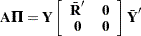

  where is lower triangular.

           ord  = j(n,1,0);
           call qr(qtb,r2,pivqr,lindqr,a,ord,b);
           nr   = n - lindqr;
           r    = r2[1:nr,]`;
           call qr(q,r5,piv2,lin2,r);
           y    = trisolv(2,r5,qtb[1:nr]);
           x6   = shape(0,n,1);
           x6[pivqr] = q * (y // j(lindqr,1,0.));
           len6 = x6` * x6;
           ss6  = ssq(a * x6 - b);
           x6   = x6`;
           print ss6 len6, x6 [format=best6.];
        

  The solution obtained by complete QR decomposition has minimum Euclidean length.

• Perform complete QR decomposition with the QR and LUPDT calls:

           ord  = j(n,1,0);
           call qr(qtb,r2,pivqr,lindqr,a,ord,b);
           nr   = n - lindqr;
           r    = r2[1:nr,1:nr]`; z = r2[1:nr,nr+1:n]`;
           call lupdt(lup,bup,sup,r,z);
           rd   = trisolv(3,lup,r2[1:nr,]);
           rd   = trisolv(4,lup,rd);
           x7   = shape(0,n,1);
           x7[pivqr] = rd` * qtb[1:nr,];
           len7 = x7` * x7;
           ss7  = ssq(a * x7 - b);
           x7 = x7`;
           print ss7 len7, x7 [format=best6.];
        

  The solution obtained by complete QR decomposition has minimum Euclidean length.

• Perform complete QR decomposition with the RUPDT, RZLIND, and LUPDT calls:

           r3 = shape(0,n,n);
           qtb = shape(0,n,1);
           call rupdt(rup,bup,sup,r3,a,qtb,b);
           r3 = rup; qtb = bup;
           call rzlind(lind,r4,bup,r3,,qtb);
           nr = n - lind; qtb = bup;
           r = r4[piv[1:nr],piv[1:nr]]`;
           z = r4[piv[1:nr],piv[nr+1:n]]`;
           call lupdt(lup,bup,sup,r,z);
           rd = trisolv(3,lup,r4[piv[1:nr],]);
           rd = trisolv(4,lup,rd);
           x8 = shape(0,n,1);
           x8 = rd` * qtb[piv[1:nr],];
           len8 = x8` * x8;
           ss8 = ssq(a * x8 - b);
           x8 = x8`;
           print ss8 len8, x8 [format=best6.];
        

  The solution obtained by complete QR decomposition has minimum Euclidean length. The same result can be obtained with the APPCORT or COMPORT call.

You can use various orthogonal methods to compute the Moore-Penrose inverse of a rectangular matrix . The entries in the following list find the Moore-Penrose inverse of the matrix shown on .

• Use the GINV operator. The GINV operator uses the singular decomposition . The result should be identical to the result given by the next solution.

           ga = ginv(a);
           t1 = a * ga; t2 = t1`;
           t3 = ga * a; t4 = t3`;
           ss1 = ssq(t1 - t2) + ssq(t3 - t4) +
                 ssq(t1 * a - a) + ssq(t3 * ga - ga);
           print ss1, ga [format=best6.];
        

• Use singular value decomposition. The singular decomposition with , , and , can be used to compute , with and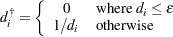

  The result should be the same as that given by the GINV operator if the singularity criterion is selected correspondingly. Since you cannot specify the criterion for the GINV operator, the singular value decomposition approach can be important for applications where the GINV operator uses an unsuitable criterion. The slight discrepancy between the values of SS1 and SS2 is due to rounding that occurs in the statement that computes the matrix GA.

           call svd(u,d,v,a);
           do i=1 to n;
              if d[i] <= 1e-10 * d[1] then d[i] = 0.;
              else d[i] = 1. / d[i];
           end;
           ga = v * diag(d) * u`;
           t1 = a * ga; t2 = t1`;
           t3 = ga * a; t4 = t3`;
           ss2 = ssq(t1 - t2) + ssq(t3 - t4) +
                 ssq(t1 * a - a) + ssq(t3 * ga - ga);
           print ss2;
        

• Use complete QR decomposition. The complete QR decomposition

  where is lower triangular, yields the Moore-Penrose inverse

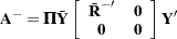
           ord = j(n,1,0);
           call qr(q1,r2,pivqr,lindqr,a,ord);
           nr = n - lindqr;
           q1 = q1[,1:nr]; r = r2[1:nr,]`;
           call qr(q2,r5,piv2,lin2,r);
           tt = trisolv(4,r5`,q1`);
           ga = shape(0,n,m);
           ga[pivqr,] = q2 * (tt // shape(0,n-nr,m));
           t1 = a * ga; t2 = t1`;
           t3 = ga * a; t4 = t3`;
           ss3 = ssq(t1 - t2) + ssq(t3 - t4) +
                 ssq(t1 * a - a) + ssq(t3 * ga - ga);
           print ss3;
        

• Use complete QR decomposition with QR and LUPDT:

           ord = j(n,1,0);
           call qr(q,r2,pivqr,lindqr,a,ord);
           nr = n - lindqr;
           r = r2[1:nr,1:nr]`; z = r2[1:nr,nr+1:n]`;
           call lupdt(lup,bup,sup,r,z);
           rd = trisolv(3,lup,r2[1:nr,]);
           rd = trisolv(4,lup,rd);
           ga = shape(0,n,m);
           ga[pivqr,] = rd` * q[,1:nr]`;
           t1 = a * ga; t2 = t1`;
           t3 = ga * a; t4 = t3`;
           ss4 = ssq(t1 - t2) + ssq(t3 - t4) +
                 ssq(t1 * a - a) + ssq(t3 * ga - ga);
           print ss4;
        

• Use complete QR decomposition with RUPDT and LUPDT:

           r3 = shape(0,n,n);
           y = i(m); qtb = shape(0,n,m);
           call rupdt(rup,bup,sup,r3,a,qtb,y);
           r3 = rup; qtb = bup;
           call rzlind(lind,r4,bup,r3,,qtb);
           nr = n - lind; qtb = bup;
           r = r4[piv[1:nr],piv[1:nr]]`;
           z = r4[piv[1:nr],piv[nr+1:n]]`;
           call lupdt(lup,bup,sup,r,z);
           rd = trisolv(3,lup,r4[piv[1:nr],]);
           rd = trisolv(4,lup,rd);
           ga = shape(0,n,m);
           ga = rd` * qtb[piv[1:nr],];
           t1 = a * ga; t2 = t1`;
           t3 = ga * a; t4 = t3`;
           ss5 = ssq(t1 - t2) + ssq(t3 - t4) +
                 ssq(t1 * a - a) + ssq(t3 * ga - ga);
           print ss5;