Time Series Analysis and Examples: Minimum AIC Procedure

Time Series Analysis and Examples

Minimum AIC Procedure

The AIC statistic is widely used to select the best model among alternative parametric models. The minimum AIC model selection procedure can be interpreted as a maximization of the expected entropy (Akaike 1981). The entropy of a true probability density function (PDF) $\varphi$ with respect to the fitted PDF is written as

$b(\varphi,f) = -i(\varphi,f)$

where $i(\varphi,f)$ is a Kullback-Leibler information measure, which is defined as

$i(\varphi,f) = \int [ \log [ \frac{\varphi(z)}{f(z)} ] ] \varphi(z) dz$

where the random variable

is assumed to be continuous. Therefore,

$b(\varphi,f) = {\rm e}_z \log f(z) - {\rm e}_z \log \varphi(z)$

where $b(\varphi,f)\leq 0$ and E

denotes the expectation concerning the random variable

. $b(\varphi,f)=0$ if and only if $\varphi=f$ (a.s.). The larger the quantity E $_z \log f(z)$ , the closer the function

is to the true PDF $\varphi$ . Given the data ${y}= (y_1, ... , y_t)^'$ that has the same distribution as the random variable

, let the likelihood function of the parameter vector $\theta$ be $\prod_{t=1}^t f(y_t|\theta)$ . Then the average of the log-likelihood function $\frac{1}t\sum_{t=1}^t \log f(y_t|\theta)$ is an estimate of the expected value of $\log f(z)$ . Akaike (1981) derived the alternative estimate of E $_z \log f(z)$ by using the Bayesian predictive likelihood. The AIC is the bias-corrected estimate of $-2t{\rm e}_z \log f(z|\hat{\theta})$ , where $\hat{\theta}$ is the maximum likelihood estimate.

${\rm aic} = - 2({maximum log-likelihood}) + 2({number of free parameters})$

Let $\theta = (\theta_1, ... ,\theta_k)^'$ be a

parameter vector that is contained in the parameter space $\theta_k$ . Given the data

, the log-likelihood function is

$\ell(\theta) = \sum_{t=1}^t \log f(y_t|\theta)$

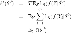
Suppose the probability density function $f(y|\theta)$ has the true PDF $\varphi(y) = f(y|\theta^0)$ , where the true parameter vector $\theta^0$ is contained in $\theta_k$ . Let $\hat{\theta}_k$ be a maximum likelihood estimate. The maximum of the log-likelihood function is denoted as $\ell(\hat{\theta}_k) = \max_{\theta\in\theta_k}\ell(\theta)$ . The expected log-likelihood function is defined by

$\ell^*(\theta) = t{\rm e}_z \log f(z|\theta)$

The Taylor series expansion of the expected log-likelihood function around the true parameter $\theta^0$ gives the following asymptotic relationship:

$\ell^*(\theta) \stackrel{a}{=} \ell^*(\theta^0) + t(\theta - \theta^0)^'{\rm e}... ...rtial \theta} - \frac{t}2(\theta - \theta^0)^' i(\theta^0)(\theta - \theta^0)$

where $i(\theta^0)$ is the information matrix and $\stackrel{a}{=}$ stands for asymptotic equality. Note that $\frac{\partial \log f(z|\theta^0)}{\partial \theta}=0$ since $\log f(z|\theta)$ is maximized at $\theta^0$ . By substituting $\hat{\theta}_k$ , the expected log-likelihood function can be written as

$\ell^*(\hat{\theta}_k) \stackrel{a}{=} \ell^*(\theta^0) - \frac{t}2(\hat{\theta}_k - \theta^0)^' i(\theta^0)(\hat{\theta}_k - \theta^0)$

The maximum likelihood estimator is asymptotically normally distributed under the regularity conditions

$\sqrt{t}i(\theta^0)^{1/2}(\hat{\theta}_k - \theta^0) \stackrel{d}{arrow}n(0, i_k)$

Therefore,

$t(\hat{\theta}_k - \theta^0)^'i(\theta^0)(\hat{\theta}_k - \theta^0) \stackrel{a}{\sim} \chi_k^2$

The mean expected log-likelihood function, $\ell^*(k) = {\rm e}_y \ell^*(\hat{\theta}_k)$ , becomes

$\ell^*(k) \stackrel{a}{=} \ell^*(\theta^0) - \frac{k}2$

When the Taylor series expansion of the log-likelihood function around $\hat{\theta}_k$ is used, the log-likelihood function $\ell(\theta)$ is written

$\ell(\theta) \stackrel{a}{=} \ell(\hat{\theta}_k) + (\theta - \hat{\theta}_k)^'... ...partial \theta \partial \theta^'} | _{\hat{\theta}_k}(\theta - \hat{\theta}_k)$

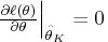
Since $\ell(\hat{\theta}_k)$ is the maximum log-likelihood function, $. \frac{\partial \ell(\theta)} {\partial \theta} | _{\hat{\theta}_k}=0$ . Note that ${\rm plim} [ -\frac{1}t . \frac{\partial^2 \ell(\theta)} {\partial \theta \partial \theta^'} | _{\hat{\theta}_k} ] = i(\theta^0)$ if the maximum likelihood estimator $\hat{\theta}_k$ is a consistent estimator of $\theta$ . Replacing $\theta$ with the true parameter $\theta^0$ and taking expectations with respect to the random variable

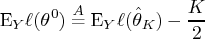
${\rm e}_y \ell(\theta^0) \stackrel{a}{=} {\rm e}_y \ell(\hat{\theta}_k) - \frac{k}2$

Consider the following relationship:

$\ell^*(\theta^0) & = & t{\rm e}_z \log f(z|\theta^0) \ & = & {\rm e}_y \sum_{t=1}^t \log f(y_t|\theta^0) \ & = & {\rm e}_y \ell(\theta^0)$

From the previous derivation,

$\ell^*(k) \stackrel{a}{=} \ell^*(\theta^0) - \frac{k}2$

Therefore,

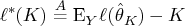
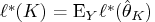
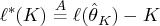
$\ell^*(k) \stackrel{a}{=} {\rm e}_y \ell(\hat{\theta}_k) - k$

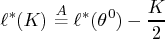
The natural estimator for E $_y \ell(\hat{\theta}_k)$ is $\ell(\hat{\theta}_k)$ . Using this estimator, you can write the mean expected log-likelihood function as

$\ell^*(k) \stackrel{a}{=} \ell(\hat{\theta}_k) - k$

Consequently, the AIC is defined as an asymptotically unbiased estimator of

${\rm aic}(k) = -2\ell(\hat{\theta}_k) + 2k$

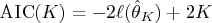
In practice, the previous asymptotic result is expected to be valid in finite samples if the number of free parameters does not exceed $2\sqrt{t}$ and the upper bound of the number of free parameters is $\frac{t}2$ . It is worth noting that the amount of AIC is not meaningful in itself, since this value is not the Kullback-Leibler information measure. The difference of AIC values can be used to select the model. The difference of the two AIC values is considered insignificant if it is far less than 1. It is possible to find a better model when the minimum AIC model contains many free parameters.

Top of Page