Nonlinear Optimization Examples: Finite-Difference Approximations of Derivatives

Nonlinear Optimization Examples

Finite-Difference Approximations of Derivatives

If the optimization technique needs first- or second-order derivatives and you do not specify the corresponding IML module "grd," "hes," "jac," or "jacnlc," the derivatives are approximated by finite-difference formulas using only calls of the module "fun." If the optimization technique needs second-order derivatives and you specify the "grd" module but not the "hes" module, the subroutine approximates the second-order derivatives by finite differences using or calls of the "grd" module.

The eighth element of the opt argument specifies the type of finite-difference approximation used to compute first- or second-order derivatives and whether the finite-difference intervals, , should be computed by an algorithm of Gill et al. (1983). The value of opt[8] is a two-digit integer, .

If opt[8] is missing or , the fast but not very precise forward-difference formulas are used; if $j \neq 0$ , the numerically more expensive central-difference formulas are used.
If opt[8] is missing or $i \neq 1,2,{ or }3$ , the finite-difference intervals are based only on the information of par[8] or par[9], which specifies the number of accurate digits to use in evaluating the objective function and nonlinear constraints, respectively. If , the intervals are computed with an algorithm by Gill et al. (1983). For , the interval is based on the behavior of the objective function; for , the interval is based on the behavior of the nonlinear constraint functions; and for , the interval is based on the behavior of both the objective function and the nonlinear constraint functions.

Forward-Difference Approximations

First-order derivatives: additional function calls are needed.
$g_i = {\partial f \over \partial x_i} = {f(x + h_ie_i) - f(x) \over h_i}$
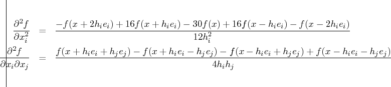
Second-order derivatives based on function calls only, when the "grd" module is not specified (Dennis and Schnabel 1983): for a dense Hessian matrix, additional function calls are needed.
${\partial^2 f \over \partial x_i \partial x_j} = {f(x+h_ie_i+h_je_j) - f(x+h_ie_i) - f(x+h_je_j) + f(x) \over h_i h_j}$
Second-order derivatives based on gradient calls, when the "grd" module is specified (Dennis and Schnabel 1983): additional gradient calls are needed.
${\partial^2 f \over \partial x_i \partial x_j} = {g_i(x + h_je_j) - g_i(x) \over 2h_j} + {g_j(x + h_ie_i) - g_j(x) \over 2h_i}$

Central-Difference Approximations

First-order derivatives: additional function calls are needed.
$g_i = {\partial f \over \partial x_i} = {f(x + h_ie_i) - f(x - h_ie_i) \over 2h_i}$
Second-order derivatives based on function calls only, when the "grd" module is not specified (Abramowitz and Stegun 1972): for a dense Hessian matrix, additional function calls are needed.
${} {\partial^2 f \over \partial x^2_i} & = & {-f(x + 2h_ie_i) + 16f(x + h_ie... ...x+h_ie_i-h_je_j) - f(x-h_ie_i+h_je_j) + f(x-h_ie_i-h_je_j) \over 4h_ih_j}$
Second-order derivatives based on gradient calls, when the "grd" module is specified: additional gradient calls are needed.
${\partial^2 f \over \partial x_i \partial x_j} = {g_i(x + h_je_j) - g_i(x - h_je_j) \over 4h_j} + {g_j(x + h_ie_i) - g_j(x - h_ie_i) \over 4h_i}$

The step sizes

, are defined as follows:

For the forward-difference approximation of first-order derivatives using only function calls and for second-order derivatives using only gradient calls, $h_j = \sqrt[2]{\eta_j} (1 + | x_j|)$ .
For the forward-difference approximation of second-order derivatives using only function calls and for central-difference formulas, $h_j = \sqrt[3]{\eta_j} (1 + | x_j|)$ .

If the algorithm of Gill et al. (1983) is not used to compute $\eta_j$ , a constant value $\eta = \eta_j$ is used depending on the value of par[8].

If the number of accurate digits is specified by par, then $\eta$ is set to $10^{-k_1}$ .
If par[8] is not specified, $\eta$ is set to the machine precision, $\epsilon$ .

If central-difference formulas are not specified, the optimization algorithm switches automatically from the forward-difference formula to a corresponding central-difference formula during the iteration process if one of the following two criteria is satisfied:

The absolute maximum gradient element is less than or equal to 100 times the ABSGTOL threshold.
The term on the left of the GTOL criterion is less than or equal to $\max(1$ E-6, GTOL threshold. The 1E-6 ensures that the switch is performed even if you set the GTOL threshold to zero.

The algorithm of Gill et al. (1983) that computes the finite-difference intervals

can be very expensive in the number of function calls it uses. If this algorithm is required, it is performed twice, once before the optimization process starts and once after the optimization terminates.

Many applications need considerably more time for computing second-order derivatives than for computing first-order derivatives. In such cases, you should use a quasi-Newton or conjugate gradient technique.

If you specify a vector, , of nonlinear constraints with the "nlc" module but you do not specify the "jacnlc" module, the first-order formulas can be used to compute finite-difference approximations of the Jacobian matrix of the nonlinear constraints.

$( \nabla c_i ) = ( \frac{\partial c_i}{\partial x_j} ) , i= 1, ... ,nc, j=1, ... ,n$

You can specify the number of accurate digits in the constraint evaluations with par[9]. This specification also defines the step sizes

Note: If you are not able to specify analytic derivatives and if the finite-difference approximations provided by the subroutines are not good enough to solve your optimization problem, you might be able to implement better finite-difference approximations with the "grd," "hes," "jac," and `` jacnlc'' module arguments.

Top of Page