Language Reference: BSPLINE Function :: SAS/IML(R) 9.2 User's Guide

Language Reference

BSPLINE Function

computes a B-spline basis

BSPLINE( , , $\lt,i\gt$ )

The inputs to the BSPLINE function are as follows:

is an

numeric vector.

is a nonnegative numeric scalar value that specifies the degree of the B-spline. Note that the order of a B-spline is one greater than the degree.

is a numeric vector of size

that contains the B-spline knots or a scalar that denotes the number of interior knots. When $n \gt 1$ , the elements of the knot vector must be nondecreasing, $k_{j-1} \leq k_{j}$ for

is an optional argument that specifies the number of interior knots when

and

contains a missing value. In this case the BSPLINE function constructs a vector of knots as follows. If $x_{(1)}$ and $x_{(m)}$ are the smallest and largest value in the

vector, then interior knots are placed at

$x_{(1)} + j(x_{(m)} - x_{(1)})/(k+1), j=1, ... ,k$

In addition,

exterior knots are placed under $x_{(1)}$ and max(

,1) exterior knots are placed over $x_{(m)}$ . The exterior knots are evenly spaced and start at $x_{(1)} -$ 1E-12 and $x_{(m)} +$ 1E-12. In this case the BSPLINE function returns a matrix with

rows and

columns.

The BSPLINE function computes B-splines of degree

. Suppose that $b_{j}^d(x)$ denotes the

th B-spline of degree

in the knot sequence

. de Boor (2001) defines the splines based on the following relationships:

$b_{j}^0(x) = \{ 1 & k_j \leq x \lt k_{j+1} \cr 0 & {otherwise} .$

and for $d \gt 0$

$b_{j}^d(x) &=& w_{j}^d(x) b_{j}^{d-1}(x) + (1-w_{j+1}^d(x)) b_{j+1}^{d-1}(x) \ w_{j}^d(x) &=& \frac{x-k_j}{k_{j+d}-k_j}$

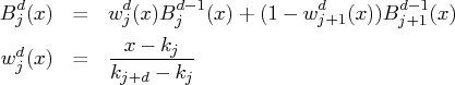
Note that de Boor (2001) expresses B-splines in terms of order rather than degree; in his notation $b_{j,d} = b_j^{d-1}$ . B-splines have many interesting properties. For example:

$\sum_j b_j^d = 1$
The sequence is positive on knots and zero elsewhere.
The B-spline is a piecewise polynomial of at most pieces.
If $k_j = k_{j+d}$ , then $b_j^{d-1} = 0$ .

See de Boor (2001) for more details. The BSPLINE function defines B-splines of degree 0 as nonzero if $k_j \lt x \leq k_{j+1}$ .

A typical knot vector for calculating B-splines consists of exterior knots smaller than the smallest data value, and $\max\{d,1\}$ exterior knots larger than the largest data value. The remaining knots are the interior knots.

For example, consider the following statements and the output they produce:

  
    x     = {2.5 3 4.5 5.1}; 
    knots = {0 1 2 3 4 5 6 7 8}; 
    bsp = bspline(x,3,knots); 
    print bsp[format=best7.];

  
    0.02083 0.47917 0.47917 0.02083       0       0       0 
          0 0.16667 0.66667 0.16667       0       0       0 
          0       0 0.02083 0.47917 0.47917 0.02083       0 
          0       0       0  0.1215 0.65717 0.22117 0.00017

In this example there are

interior knots and the BSPLINE function returns a matrix with

columns. If you pass an

vector of data values, you can also rely on the BSPLINE function to compute a knot vector for you. For example, the following statements produce B-splines of degree 2 based on 4 equally spaced interior knots:

  
    n = 20; 
    x = ranuni(J(n,1,45)); 
    bsp = bspline(x,2,.,4); 
    print bsp[format=8.3];

The resulting matrix is as follows:

  
     0.000    0.104    0.748    0.147    0.000    0.000    0.000 
     0.000    0.000    0.000    0.286    0.684    0.030    0.000 
     0.000    0.000    0.000    0.000    0.000    0.517    0.483 
     0.000    0.000    0.000    0.217    0.725    0.058    0.000 
     0.000    0.000    0.239    0.713    0.048    0.000    0.000 
     0.000    0.000    0.000    0.446    0.553    0.002    0.000 
     0.000    0.000    0.394    0.600    0.006    0.000    0.000 
     0.000    0.000    0.000    0.000    0.064    0.729    0.207 
     0.000    0.389    0.604    0.007    0.000    0.000    0.000 
     0.000    0.000    0.000    0.000    0.000    0.500    0.500 
     0.000    0.000    0.000    0.000    0.210    0.728    0.062 
     0.000    0.000    0.014    0.639    0.347    0.000    0.000 
     0.000    0.001    0.546    0.453    0.000    0.000    0.000 
     0.500    0.500    0.000    0.000    0.000    0.000    0.000 
     0.304    0.672    0.024    0.000    0.000    0.000    0.000 
     0.000    0.020    0.659    0.322    0.000    0.000    0.000 
     0.000    0.277    0.690    0.033    0.000    0.000    0.000 
     0.386    0.606    0.007    0.000    0.000    0.000    0.000 
     0.000    0.000    0.000    0.000    0.022    0.667    0.311 
     0.008    0.612    0.380    0.000    0.000    0.000    0.000

Top of Page