Language Reference: KALCVS Call :: SAS/IML(R) 9.2 User's Guide

Language Reference

KALCVS Call

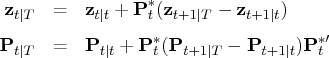
uses backward recursions to compute the smoothed estimate ${z}_{t| t}$ and its covariance matrix, ${p}_{t| t}$ , where is the number of observations in the complete data set

CALL KALCVS( sm, vsm, data, , , , , var, pred, vpred <,un, vun>);

The inputs to the KALCVS subroutine are as follows.

data: is a matrix containing data $({y}_1, ... , {y}_t)^'$ .
: is an vector for a time-invariant input vector in the transition equation, or a vector containing input vectors in the transition equation.
: is an matrix for a time-invariant transition matrix in the transition equation, or a matrix containing transition matrices.
: is an vector for a time-invariant input vector in the measurement equation, or a vector containing input vectors in the measurement equation.
: is an matrix for a time-invariant measurement matrix in the measurement equation, or a matrix containing time-variant ${h}_t$ matrices in the measurement equation.
var: is an covariance matrix for the errors in the transition and the measurement equations, or a matrix containing covariance matrices in the transition equation and measurement equation noises - that is, $(\eta^'_t, \epsilon^'_t)^'$ .
pred: is a matrix containing one-step forecasts $({z}_{1|}, ... , {z}_{t| t-1})^'$ .
vpred: is a matrix containing mean square error matrices of predicted state vectors $({p}_{1|}, ... , {p}_{t| t-1})^'$ .
un: is an optional vector containing ${u}_t$ . The returned value is ${u}_0$ .
vun: is an optional matrix containing ${u}_t$ . The returned value is ${u}_0$ .

The KALCVS call returns the following values:

sm: is a matrix containing smoothed state vectors $({z}_{1| t}, ... , {z}_{t| t})^'$ .
vsm: is a matrix containing covariance matrices of smoothed state vectors $({p}_{1| t}, ... , {p}_{t| t})^'$ .

When the Kalman filtering is performed in the KALCVF call, the KALCVS call computes smoothed state vectors and their covariance matrices. The fixed-interval smoothing state vector at time

is obtained by the conditional expectation given all observations.

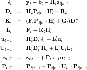
The smoothing algorithm uses one-step forecasts and their covariance matrices, which are given in the KALCVF call. For notation, ${z}_{t| t}$ is the smoothed value of the state vector ${z}_t$ , and the mean square error matrix is denoted ${p}_{t| t}$ . For smoothing,

$\hat{\epsilon}_t & = & {y}_t - {b}_t - {h}_t {z}_{t| t-1} \ {d}_t & = & {h}_t ... ...{t-1} \ {p}_{t| t} & = & {p}_{t| t-1} - {p}_{t| t-1} {u}_{t-1} {p}_{t| t-1}$

where

. The initial values are ${u}_t = 0$ and ${u}_t = 0$ .

When the SSM is specified by using the alternative transition equation

${z}_t = {a}_t + {f}_t{z}_{t-1} + \eta_t$

the fixed-interval smoothing is performed by using the following backward recursions:

$\hat{\epsilon}_t & = & {y}_t - {b}_t - {h}_t {z}_{t| t-1} \ {d}_t & = & {h}_t ... ...{t-1} \ {p}_{t| t} & = & {p}_{t| t-1} - {p}_{t| t-1} {u}_{t-1} {p}_{t| t-1}$

where it is assumed that ${g}_t = 0$ .

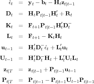
You can use the KALCVS call regardless of the specification of the transition equation when ${g}_t = 0$ . Harvey (1989) gives the following fixed-interval smoothing formula, which produces the same smoothed value:

${z}_{t| t} & = & {z}_{t| t} + {p}^*_t ({z}_{t+1| t} - {z}_{t+1| t}) \ {p}_{t| t} & = & {p}_{t| t} + {p}^*_t ({p}_{t+1| t} - {p}_{t+1| t}) {p}^{*'_t$

where

${p}^*_t = {p}_{t| t} {f}^'_t {p}^-_{t+1| t}$

under the shifted transition equation, but

${p}^*_t = {p}_{t| t} {f}^'_{t+1} {p}_{t+1| t}^-$

under the alternative transition equation.

The KALCVS call is accompanied by the KALCVF call, as shown in the following code. Note that you do not need to specify UN and VUN.

  
    call kalcvf(pred,vpred,filt,vfilt,y,0,a,f,b,h,var); 
    call kalcvs(sm,vsm,y,a,f,b,h,var,pred,vpred);

You can also compute the smoothed estimate and its covariance matrix on an observation-by-observation basis. When the SSM is time invariant, the following example performs smoothing. In this situation, you should initialize UN and VUN as matrices of value 0, as in the following code:

  
 call kalcvf(pred,vpred,filt,vfilt,y,0,a,f,b,h,var); 
 n = nrow(y); 
 nz = ncol(f); 
 un = j(1,nz,0); 
 vun = j(nz,nz,0); 
 do i = 1 to n; 
   y_i = y[n-i+1,]; 
   pred_i  = pred[n-i+1,]; 
   vpred_i = vpred[(n-i)*nz+1:(n-i+1)*nz,]; 
   call kalcvs(sm_i,vsm_i,y_i,a,f,b,h,var,pred_i,vpred_i,un,vun); 
   sm  = sm_i // sm; 
   vsm = vsm_i // vsm; 
 end;

The KALCVF call has an example program that includes the KALCVS call.

Top of Page