| Language Reference |
KALCVF Call
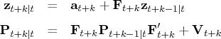
computes the one-step prediction
![]() and the filtered estimate
and the filtered estimate
![]() , as well as their covariance matrices.
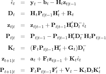
The call uses forward recursions, and you
can also use it to obtain
, as well as their covariance matrices.
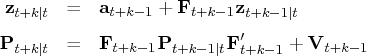
The call uses forward recursions, and you
can also use it to obtain ![]() -step estimates.
-step estimates.
- CALL KALCVF( pred, vpred, filt, vfilt, data, lead,
 ,
,  ,
,  ,
,  ,
,
- var <, z0, vz0>);
The inputs to the KALCVF subroutine are as follows:
- data
- is a
 matrix containing data
 .
. - lead
- is the number of steps to forecast after the end of the data.
- is an
 vector for a time-invariant input vector in
the transition equation, or a
vector for a time-invariant input vector in
the transition equation, or a  vector containing input vectors in the transition equation.
- is an
 matrix for a time-invariant
transition matrix in the transition equation, or a
matrix for a time-invariant
transition matrix in the transition equation, or a
 matrix containing
transition matrices in the transition equation.
matrix containing
transition matrices in the transition equation.
- is an
 vector for a time-invariant input vector in
the measurement equation, or a
vector for a time-invariant input vector in
the measurement equation, or a  vector containing input vectors in the measurement equation.
- is an
 matrix for a time-invariant
measurement matrix in the measurement equation, or a
matrix for a time-invariant
measurement matrix in the measurement equation, or a
 matrix containing
measurement matrices in the measurement equation.
matrix containing
measurement matrices in the measurement equation.
- var
- is an
 matrix for a
time-invariant variance matrix for the error in the transition
equation and the error in the measurement equation, or a
matrix for a
time-invariant variance matrix for the error in the transition
equation and the error in the measurement equation, or a
 matrix
containing variance matrices for the error in the transition
equation and the error in the measurement equation -
that is,
matrix
containing variance matrices for the error in the transition
equation and the error in the measurement equation -
that is,  .
. 
- is an optional
 initial
state vector
initial
state vector  .
. 
- is an optional covariance
matrix of an initial state vector
 .
.
- pred
- is a
 matrix containing
one-step predicted state vectors
matrix containing
one-step predicted state vectors  .
. - vpred
- is a matrix
containing mean square errors of predicted state
vectors
 .
. - filt
- is a
 matrix containing filtered state
vectors
matrix containing filtered state
vectors  .
. - vfilt
- is a
 matrix containing mean square errors of
filtered state vectors
matrix containing mean square errors of
filtered state vectors  .
.
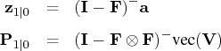
The initial state vector and its covariance matrix of the time invariant Kalman filters are computed under the stationarity condition
The KALCVF call accepts missing values in observations. If there is a missing observation, the filtered state vector for the missing observation is given by the one-step forecast.
The following program gives an example of the KALCVF call:
    q=2;
    p=2;
    n=10;
    lead=3;

    total=n+lead;

    seed = 25735;
    x=round(10*normal(j(n,p,seed)))/10;
    f=round(10*normal(j(q*total,q,seed)))/10;
    a=round(10*normal(j(total*q,1,seed)))/10;
    h=round(10*normal(j(p*total,q,seed)))/10;
    b=round(10*normal(j(p*total,1,seed)))/10;
    do i = 1 to total;
    temp=round(10*normal(j(p+q,p+q,seed)))/10;
    var=var//(temp*temp`);
    end;

    call kalcvf(pred,vpred,filt,vfilt,x,lead,a,f,b,h,var);

    /* default initial state and covariance */
    call kalcvs(sm,vsm,x,a,f,b,h,var,pred,vpred);
    print sm [format=9.4] vsm [format=9.4];
This program produces the following output:
                SM                 VSM

           -1.5236   -0.1000    1.5813   -0.4779
            0.3058   -0.1131   -0.4779    0.3963
           -0.2593    0.2496    2.4629    0.2426
           -0.5533    0.0332    0.2426    0.0944
           -0.5813    0.1251    0.2023   -0.0228
           -0.3017    0.7480   -0.0228    0.5799
            1.1333   -0.2144    0.8615   -0.7653
            1.5193   -0.6237   -0.7653    1.2334
           -0.6641   -0.7770    1.0836    0.8706
            0.5994    2.3333    0.8706    1.5252
                                0.3677    0.2510
                                0.2510    0.2051
                                0.3243   -0.4093
                               -0.4093    1.2287
                                0.1736   -0.0712
                               -0.0712    0.9048
                                1.3153    0.8748
                                0.8748    1.6575
                                8.6650    0.1841
                                0.1841    4.4770
Copyright © 2009 by SAS Institute Inc., Cary, NC, USA. All rights reserved.