Adding Insets to Classification Panels
This section requires familiarity
with Using Classification Panels. You should skip this section if you are not familiar with the general
coding for classification panels.
The DATALATTICE and DATAPANEL layouts provide INSET= and INSETOPTS=
options for displaying insets in classification panels. The INSETOPTS=
option supports the same placement and appearance features as those
documented for the SCATTERPLOTMATRIX statement in Adding Insets to a SCATTERPLOTMATRIX Graph. However, unlike
the SCATTERPLOTMATRIX statement, the DATALATTICE and DATAPANEL layouts
do not have predefined information available. Thus, for the INSET=
option, you must create the columns for the information that you want
to display in the inset and integrate it with the input data before
the graph is rendered. Then, on the INSET= option, you specify the
name(s) of the column(s) that contain the desired information.
For example, the following
template code uses INSET=(NOBS MEAN) to reference input data columns
that are named NOBS and MEAN. When the graph is rendered, the values
that are stored in these columns will be displayed in the inset.
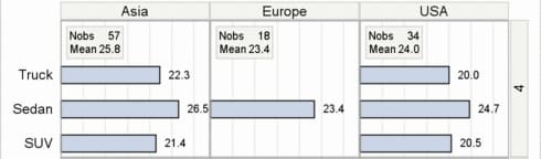
In the inset display
in this example, one row is displayed for each column that is listed
on INSET=, and each row has two columns. The left column shows the
column name (column label, if it is defined in the data), and the
right column contains the column value for that particular cell of
the panel. The number of rows of data for these columns should match
the number of cells in the classification panel and the sequence in
which the cells are populated.
The following template
code defines a template named PANEL. The template "makes room" for
the insets in each panel by adding a maximum row axis offset. In this
case, OFFSETMAX=0.4 is sufficient, but the setting will vary case-by-case.
This is what the first row of the classification panel with insets
will look like:
proc template;
define statgraph panel;
begingraph;
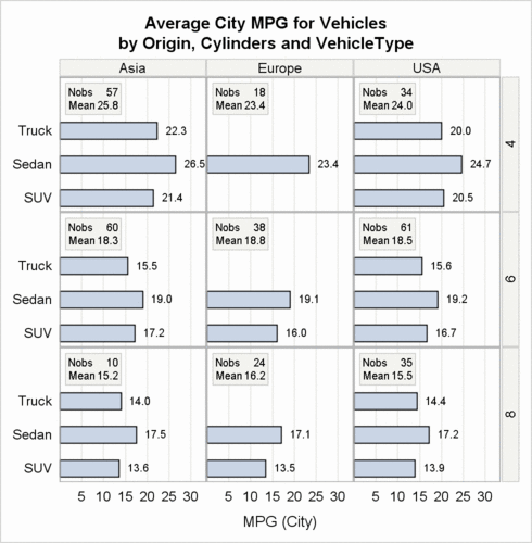
entrytitle "Average City MPG for Vehicles";
entrytitle "by Origin, Cylinders and VehicleType";
layout datalattice columnvar=origin rowvar=cylinders /
columndatarange=unionall rowdatarange=unionall
headerlabeldisplay=value
headerbackgroundcolor=GraphAltBlock:color
inset=(cellN cellMean)
insetopts=(border=true
opaque=true backgroundcolor=GraphAltBlock:color)
rowaxisopts=( offsetmax=.4 offsetmin=.1 display=(tickvalues) )
columnaxisopts=(display=(label tickvalues)
linearopts=( tickvaluepriority=true
tickvaluesequence=(start=5 end=30 increment=5))
griddisplay=on offsetmin=0 offsetmax=.1);
layout prototype;
barchart x=type y=mean / orient=horizontal
barwidth=.5 barlabel=true;
endlayout;
endlayout;
endgraph;
end;
run;
The data for this example
is from the SASHELP.CARS data set. To calculate the number of observations
and mean for the observations, we can use PROC SUMMARY.
The following PROC SUMMARY
step calculates the number of observations and the mean of MPG_CITY
for each of the classification interactions listed in the TYPES statement.
CYLINDERS*ORIGIN is the crossing needed for the cell summaries, and
CYLINDER*ORIGIN*TYPE is the crossing needed by each cell's bar chart.
The COMPLETETYPES option
creates summary observations even when the frequency of the classification
interactions is zero. Additionally, the code creates subsets in the
input data to restrict the number of bars in each bar chart to at
most three, and to reduce the number cells in the classification panel.
There are three values of ORIGIN (Asia, Europe, and USA) and three
values of CYLINDERS (4, 6, and 8).
For the insets to display
accurate data, we must ensure that the order of the observations in
the data corresponds to the column order for the CLASS statement of
PROC SUMMARY. Because the panel cells are populated across one row
before proceeding to the next row, the values of the panel's row variable
(CYLINDERS) determines the panel order and must be specified first
in the SUMMARY procedure's CLASS statement so that the values of CYLINDERS
also determine the order for the statistics calculations.
/* compute the barchart data and inset information */

proc summary data=sashelp.cars completetypes;
  where type in ("Sedan" "Truck" "SUV") and
        cylinders in (4 6 8);
  class cylinders origin type;
  var mpg_city;
  output out=mileage mean=Mean n=Nobs / noinherit;
  types cylinders*origin cylinders*origin*type;
run;
NOTE: There were 337 observations read from the data set SASHELP.CARS.
      WHERE type in ('SUV', 'Sedan', 'Truck') and cylinders in (4, 6, 8);
NOTE: The data set WORK.MILEAGE has 36 observations and 6 variables.
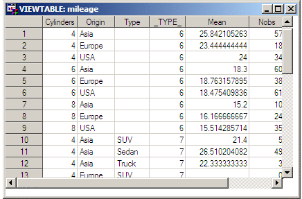
Confirm the Order of Data Observations shows the order of observations in
the interim data set named MILEAGE. Notice that the first nine observations
(where _TYPE_ equals 6) are the cell summaries. The remaining 27 observations
(where _TYPE_ equals 7) are for each cell's bar chart.
To create separate columns
for the inset, we need to store the _TYPE_= 6 observations in new
columns. The following DATA step writes the inset information to another
data set named OVERALL.
data mileage
     overall(keep=origin cylinders mean nobs
         rename=(origin=cellOrigin cylinders=cellCyl
                 mean=cellMean nobs=cellNobs ));
  set mileage; by _type_;
  if _type_ eq 6 then output overall;
  else output mileage;
run;
NOTE: There were 36 observations read from the data set WORK.MILEAGE.
NOTE: The data set WORK.MILEAGE has 27 observations and 5 variables.
NOTE: The data set WORK.OVERALL has 9 observations and 4 variables.
Finally, we create a
new data set named SUMMARY, which merges the MILEAGE and OVERALL data
sets. Note that this is a non-match merge (no BY statement), and that
all columns in the two tables have unique names to prevent overwriting
any data values.
NOTE: There were 27 observations read from the data set WORK.MILEAGE.
NOTE: There were 9 observations read from the data set WORK.OVERALL.
NOTE: The data set WORK.SUMMARY has 27 observations and 9 variables.
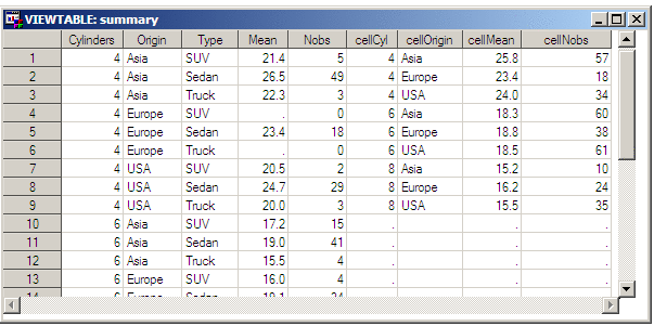
The SUMMARY data set
can now be used to render a graph from template PANEL:
ods html style=statistical;
proc sgrender data=summary template=panel;
run;
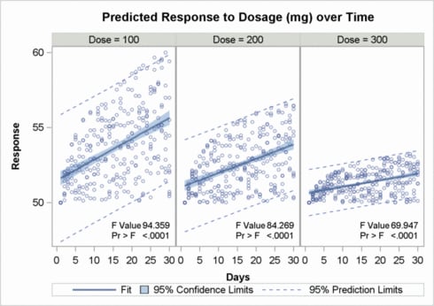
The following figure
shows another example of adding insets to a classification panel.
The complete code for this output is presented in Using Classification Panels.