Creating an Inset from Values that are Passed to the Template :: SAS(R) 9.3 Graph Template Language: User's Guide

Overview of Importing Data Into a Template

When the statistic that you want to display in an inset cannot be computed within the template, you can create an output data set from a procedure and then use dynamics or macro variables to "import" the computed values at run time.

The following discussion explains how to create and call a macro that can pass a data set name and variable name to a previously compiled GTL template. To follow this discussion, you should understand the topics that are discussed in Using Dynamics and Macro Variables to Make Flexible Templates.

For this example, we create a macro named HISTOGRAM that takes two arguments.

The first argument, DSN, passes a data set name.
The second argument, VAR, passes a variable name.

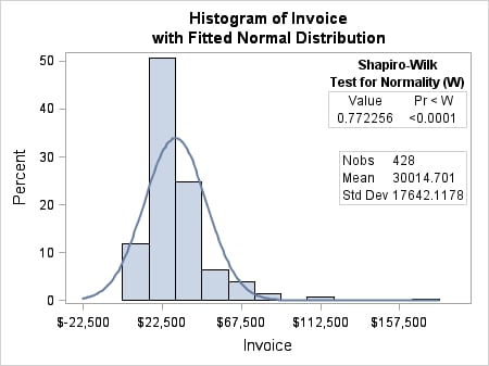
When invoked, the macro generates a histogram and model fit plot for the analysis variable VAR. The graph also displays two insets that show the related statistics.

The following call to the HISTOGRAM macro uses the data set SASHELP.HEART to generate a histogram for variable MRW (Metropolitan Relative Weight for subjects in a heart study):

%histogram(sashelp.heart, mrw)

Passing Parameter Values to a Template

For more information about creating and calling macros, see the SAS Macro Language: Reference.

Creating a Template that Uses Macro Variables

This section creates a GTL template that can generate the histogram and model fit plot that is shown in Passing Parameter Values to a Template.The template definition uses the MVAR statement to define macro variables that provide run-time values and labels for the graph insets. The MVAR statement also defines a macro variable named VAR, which is used as the column argument for the histogram and overlaid normal density plot.

For this example, the inset statistics are calculated in the macro body, and the value for macro variable VAR is passed as a parameter on the macro call.

Here is the GTL code for a template that we name GINSET:

proc template;
define statgraph  ginset;
  MVAR VAR NOBS MEAN STD TEST TESTLABEL STAT PTYPE PVALUE ;
  begingraph;
    entrytitle "Histogram of " eval(colname(VAR));
    entrytitle "with Fitted Normal Distribution";
    layout overlay;
      histogram VAR ;
      densityplot VAR / normal();
 
      /* inset for normality test */
      layout gridded / columns=1  opaque=true
             autoalign=(topright topleft);
        entry TEST / textattrs=(weight=bold);
        entry "Test for Normality " TESTLABEL /
             textattrs=(weight=bold);
        layout gridded / columns=2   border=true;
          entry "Value"; entry PTYPE ;
          entry STAT;    entry  PVALUE ;
        endlayout;
      endlayout;

      /* inset for descriptive statistics */
      layout gridded / columns=2 border=true
             opaque=true autoalign=(right left);
        entry halign=left "Nobs";    entry halign=left NOBS ;
        entry halign=left "Mean";    entry halign=left MEAN ;
        entry halign=left "Std Dev"; entry halign=left STD ;
      endlayout;
    endlayout;
  endgraph;
end;
run;

The MVAR statement declares the macro variables that will be referenced in the template.
The ENTRYTITLE statement specifies macro variable VAR as the argument on the COLNAME function, which returns the case-sensitive name of the column. Thus, the variable name that you pass on the macro call will be displayed in the graph title.
The HISTOGRAM and DENSITYPLOT statements specify macro variable VAR as their column arguments. Again, the variable name that you pass on the macro call will determine that column name.
The first LAYOUT GRIDDED block constructs a table to use as an inset. The inset identifies the normality test that is used in the analysis, and it displays the related probability statistic.

The first two ENTRY statements in the layout block specify a title for the inset. Macro variable TEST, which will be initialized by the code in the macro body, identifies the normality test that is applied to the data. As we will see later when we create the macro, either of two normality tests will be used, depending on the number of observations that are read from the data. Macro variable TESTLABEL provides either of two test labels, depending on which test is used at run time.

The nested LAYOUT GRIDDED statement defines a two-column table for the statistics table that is displayed in the first inset. Macro variable STAT in the first column provides the normality value, and macro variables PTYPE and PVALUE provide the probability statistics. These macro variables will be initialized by the code in the macro body.
The last LAYOUT GRIDDED statement constructs a two-column inset that shows descriptive statistics for the analysis variable. Macro variables NOBS, MEAN, and STD will be calculated by the code in the macro body and will resolve to the number of observations in the data, the mean value, and the standard deviation.

Defining a Macro to Initialize the Variables and Generate the Graph

In Creating a Template that Uses Macro Variables we created template GINSET, which declared the following macro variables:

TEST	Identifies the normality test that is applied to the data.
TESTLABEL	Provides the label that is associated with the applied normality test.
STAT	Provides the normality statistic that is calculated by the applied normality test.
PTYPE and PVALUE	Provide the probability (type and value) for the applied normality test.
NOBS, MEAN, and STD	Provide the number of observations, mean, and standard deviation for the analysis variable.

To initialize these macro variables, we will now create a macro that calculates values for them and also specifies an SGRENDER procedure that uses template GINSET. The macro needs two parameters: one for passing a SAS data set name, and a second for passing the name of a column in that data set.

The following macro code uses PROC UNIVARIATE to create two output data sets. A DATA step then reads the output data sets, creates the required macro variables, and assigns values to those macro variables in a local symbol table. When the macro runs the SGRENDER procedure, the values of the macro variables are imported into the GINSET template to produce a graph with insets, similar to the graph in shown in Passing Parameter Values to a Template. As mentioned earlier, the normality test that is performed on the analysis variable will be based on the number of observations in that analysis variable.

Note: To make the following macro more robust, it could be designed to validate the parameters.

%macro histogram(dsn,var);

/* compute tests for normality */
ods output TestsForNormality=norm;
proc univariate data=&dsn normaltest;
 var &var;
 output out=stats n=n mean=mean std=std;
run;

%local nobs mean std test testlabel stat ptype pvalue;
 
data _null_;
  set stats(keep=n mean std);
  call symputx("nobs",n);
  call symput("mean",strip(put(mean,12.3)));
  call symput("std",strip(put(std,12.4)));
  if n > 2000 then /* use Shapiro-Wilk */
    set norm(where=(TestLab="D"));
  else /* use Kolmogorov-Smirnov */
    set norm(where=(TestLab="W"));
  call symput("testlabel","("||trim(testlab)||")");
  call symput("test",strip(test));
  call symput("ptype",strip(ptype));
  call symput("stat",strip(put(stat,best8.)));
  call symput("pvalue",psign||put(pvalue,pvalue6.4));
run;
 
proc sgrender data=&dsn template=ginset;
run;

%mend;

The %MACRO statement declares a macro named HISTOGRAM that takes two parameters: DSN (for the data set name) and VAR (for the column name).
The ODS OUTPUT statement produces a SAS data set named NORM from the TestsForNormality output object that will be generated by the UNIVARIATE procedure (next statement). For more information about the ODS OUTPUT statement, see the SAS Output Delivery System: User's Guide.
Deriving the input data set name from the DSN parameter and the analysis variable name from the VAR parameter, the UNIVARIATE procedure calculates the number of observations, mean, and standard deviation for the analysis variable. It writes the values for these statistics to an output data set named STATS, storing the values in variables named N, MEAN, and STD.
The %LOCAL statement creates a set of local macro variables to add to the local symbol table.
The DATA step reads variables N, MEAN, and STD from the STATS data set.
The first three CALL SYMPUT routines use the data input variables to assign labels and values to the local macro variables N, MEAN, and STD. On each CALL SYMPUT, the first argument identifies the macro variable to receive the value, and the second argument identifies the data input variable that contains the value to assign to the macro variable in the symbol.
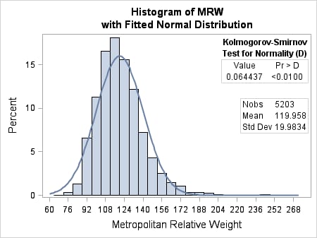
The IF/ELSE structure determines which normality test values to read from the NORM data set that was created by the ODS OUTPUT statement. If there are fewer than 2000 observations, the Shapiro-Wilk test values are used; otherwise, the Kolmogorov-Smirnov values are used.
The remaining CALL SYMPUT routines assign values to the rest of the macro variables, using the values from variables in the NORM data set.

Executing the Macro

To execute the HISTOGRAM macro, we must pass it a data set name and the name of a numeric column in the data.

The following macro call passes the data set name SASHELP.HEART and the column name MRW. Because variable MRW has more than 2000 observations, the Kolmogorov-Smirnov test is used in the analysis.

%histogram(sashelp.heart, mrw)

This next macro call passes the data set name SASHELP. CARS and the column name INVOICE. Because variable INVOICE has 2000 or fewer observations, the Shapiro-Wilk test is used in the analysis.

%histogram(sashelp.cars,invoice)

Macro Call with 2000 or Fewer Observations