The X11 Procedure
- Overview
-
Getting Started

-
Syntax
-
DetailsHistorical Development of X-11Implementation of the X-11 Seasonal Adjustment MethodComputational Details for Sliding Spans AnalysisData RequirementsMissing ValuesPrior Daily Weights and Trading-Day RegressionAdjustment for Prior FactorsThe YRAHEADOUT OptionEffect of Backcast and Forecast LengthDetails of Model SelectionOUT= Data SetThe OUTSPAN= Data SetOUTSTB= Data SetOUTTDR= Data SetPrinted OutputODS Table Names
-
Examples
- References
Example 43.3 Outlier Detection and Removal
PROC X11 can be used to detect and replace outliers in the irregular component of a monthly or quarterly series.
The weighting scheme used in measuring the "extremeness" of the irregulars is developed iteratively; thus the statistical properties of the outlier adjustment method are unknown.
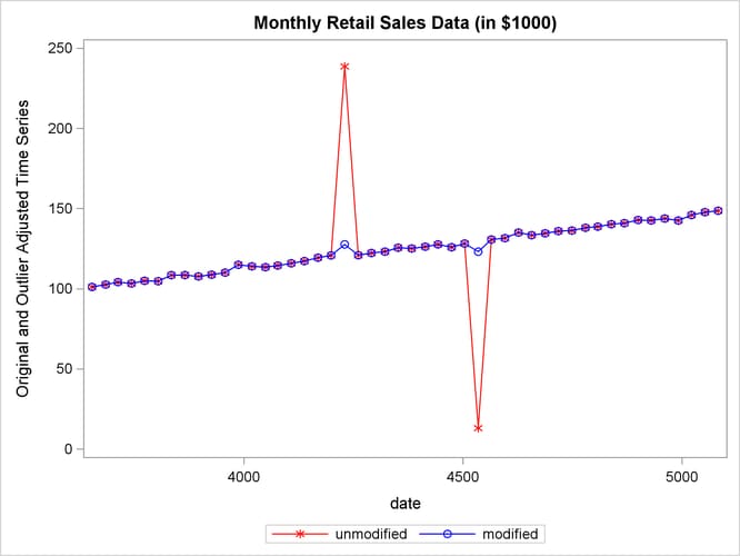
In this example, the data are simulated by generating a trend plus a random error. Two periods in the series were made "extreme" by multiplying one generated value by 2.0 and another by 0.10. The additive model is appropriate based on the way the data were generated. Note that the trend in the generated data was modeled automatically by the trend cycle component estimation.
The detection of outliers is accomplished by considering Table D9, the final replacement values for extreme S-I ratios. This table indicates which observations had irregular component values more than FULLWEIGHT= standard deviation units from 0.0 (1.0 for the multiplicative model). The default value of the FULLWEIGHT= option is 1.5; a larger value would result in fewer observations being declared extreme.
In this example, FULLWEIGHT=3.0 is used to isolate the extreme inflated and deflated values generated in the DATA step. The value of ZEROWEIGHT= must be greater than FULLWEIGHT; it is given a value of 3.5.
A plot of the original and modified series, Output 43.3.2, shows that the deviation from the trend line for the modified series is greatly reduced compared with the original series.
data a;
   retain seed 99831;
   do kk = 1 to 48;
      x = kk + 100 + rannor( seed );
      date = intnx( 'month', '01jan1970'd, kk-1 );
      if kk = 20 then x = 2 * x;
      else if kk = 30 then x = x / 10;
      output;
      end;
run;
proc x11 data=a;
   monthly date=date additive
           fullweight=3.0 zeroweight=3.5;
   var x;
   table d9;
   output out=b b1=original e1=e1;
run;

proc sgplot data=b;
   series x=date y=original / markers
                            markerattrs=(color=red symbol='asterisk')
                            lineattrs=(color=red)
                            legendlabel="unmodified" ;
   series x=date y=e1       / markers
                            markerattrs=(color=blue symbol='circle')
                            lineattrs=(color=blue)
                            legendlabel="modified" ;
   yaxis label='Original and Outlier Adjusted Time Series';
run;
Output 43.3.1: Detection of Extreme Irregulars
| Monthly Retail Sales Data (in $1000) |
| D9 Final Replacement Values for Extreme SI Ratios | ||||||||||||
|---|---|---|---|---|---|---|---|---|---|---|---|---|
| Year | JAN | FEB | MAR | APR | MAY | JUN | JUL | AUG | SEP | OCT | NOV | DEC |
| 1970 | . | . | . | . | . | . | . | . | . | . | . | . |
| 1971 | . | . | . | . | . | . | . | 11.180 | . | . | . | . |
| 1972 | . | . | . | . | . | -10.671 | . | . | . | . | . | . |
| 1973 | . | . | . | . | . | . | . | . | . | . | . | . |
Output 43.3.2: Plot of Modified and Unmodified Values