The X11 Procedure
- Overview
-
Getting Started

-
Syntax
-
DetailsHistorical Development of X-11Implementation of the X-11 Seasonal Adjustment MethodComputational Details for Sliding Spans AnalysisData RequirementsMissing ValuesPrior Daily Weights and Trading-Day RegressionAdjustment for Prior FactorsThe YRAHEADOUT OptionEffect of Backcast and Forecast LengthDetails of Model SelectionOUT= Data SetThe OUTSPAN= Data SetOUTSTB= Data SetOUTTDR= Data SetPrinted OutputODS Table Names
-
Examples
- References
Printed Output
The output from PROC X11, both printed tables and the series written to the OUT= data set, depends on whether the data are monthly or quarterly. For the printed tables, the output depends further on the value of the PRINTOUT= option and the TABLE statement, along with other options specified.
The printed output is organized into tables identified by a part letter and a sequence number within the part. The seven major parts of the X11 procedure are as follows:
- A
-
prior adjustments (optional)
- B
-
preliminary estimates of irregular component weights and regression trading-day factors
- C
-
final estimates of irregular component weights and regression trading-day factors
- D
-
final estimates of seasonal, trend cycle, and irregular components
- E
-
analytical tables
- F
-
summary measures
- G
-
charts
Table 43.3 describes the individual tables and charts. Most tables apply both to quarterly and monthly series. Those that apply only to a monthly time series are indicated by an "M" in the notes section, while "P" indicates the table is not a time series, and is only printed, not output to the OUT= data set.
Table 43.3: Table Names and Descriptions
|
Table |
Description |
Notes |
|---|---|---|
|
A1 |
original series |
M |
|
A2 |
prior monthly adjustment factors |
M |
|
A3 |
original series adjusted for prior monthly factors |
M |
|
A4 |
prior trading-day adjustments |
M |
|
A5 |
prior adjusted or original series |
M |
|
A13 |
ARIMA forecasts |
|
|
A14 |
ARIMA backcasts |
|
|
A15 |
prior adjusted or original series extended by ARIMA backcasts and forecasts |
|
|
B1 |
prior adjusted or original series |
|
|
B2 |
trend cycle |
|
|
B3 |
unmodified seasonal-irregular (S-I) ratios |
|
|
B4 |
replacement values for extreme S-I ratios |
|
|
B5 |
seasonal factors |
|
|
B6 |
seasonally adjusted series |
|
|
B7 |
trend cycle |
|
|
B8 |
unmodified S-I ratios |
|
|
B9 |
replacement values for extreme S-I ratios |
|
|
B10 |
seasonal factors |
|
|
B11 |
seasonally adjusted series |
|
|
B13 |
irregular series |
|
|
B14 |
extreme irregular values excluded from trading-day regression |
M |
|
B15 |
preliminary trading-day regression |
M,P |
|
B16 |
trading-day adjustment factors |
M |
|
B17 |
preliminary weights for irregular components |
|
|
B18 |
trading-day factors derived from combined daily weights |
M |
|
B19 |
original series adjusted for trading-day and prior variation |
M |
|
C1 |
original series modified by preliminary weights and adjusted for trading-day and prior variation |
|
|
C2 |
trend cycle |
|
|
C4 |
modified S-I ratios |
|
|
C5 |
seasonal factors |
|
|
C6 |
seasonally adjusted series |
|
|
C7 |
trend cycle |
|
|
C9 |
modified S-I ratios |
|
|
C10 |
seasonal factors |
|
|
C11 |
seasonally adjusted series |
|
|
C13 |
irregular series |
|
|
C14 |
extreme irregular values excluded from trading-day regression |
M |
|
C15 |
final trading-day regression |
M,P |
|
C16 |
final trading-day adjustment factors derived from regression coefficients |
M |
|
C17 |
final weight for irregular components |
|
|
C18 |
final trading-day factors derived from combined daily weights |
M |
|
C19 |
original series adjusted for trading-day and prior variation |
M |
|
D1 |
original series modified for final weights and adjusted for trading-day and prior variation |
|
|
D2 |
trend cycle |
|
|
D4 |
modified S-I ratios |
|
|
D5 |
seasonal factors |
|
|
D6 |
seasonally adjusted series |
|
|
D7 |
trend cycle |
|
|
D8 |
final unmodified S-I ratios |
|
|
D9 |
final replacement values for extreme S-I ratios |
|
|
D10 |
final seasonal factors |
|
|
D11 |
final seasonally adjusted series |
|
|
D12 |
final trend cycle |
|
|
D13 |
final irregular series |
|
|
E1 |
original series with outliers replaced |
|
|
E2 |
modified seasonally adjusted series |
|
|
E3 |
modified irregular series |
|
|
E4 |
ratios of annual totals |
P |
|
E5 |
percent changes in original series |
|
|
E6 |
percent changes in final seasonally adjusted series |
|
|
F1 |
MCD moving average |
|
|
F2 |
summary measures |
P |
|
G1 |
chart of final seasonally adjusted series and trend cycle |
P |
|
G2 |
chart of S-I ratios with extremes, S-I ratios without extremes, and final seasonal factors |
P |
|
G3 |
chart of S-I ratios with extremes, S-I ratios without extremes, and final seasonal factors in calendar order |
P |
|
G4 |
chart of final irregular and final modified irregular series |
P |
The PRINTOUT= Option
The PRINTOUT= option controls printing for groups of tables. See the TABLES Statement for details on specifying individual tables. The following list gives the tables printed for each value of the PRINTOUT= option:
- STANDARD (26 tables)
-
A1–A4, B1, C13–C19, D8–D13, E1–E6, F1, F2
- LONG (40 tables)
-
A1–A5, A13–A15, B1, B2, B7, B10, B13–B15, C1, C7, C10, C13–C19, D1, D7–D11, D13, E1–E6, F1, F2
- FULL (62 tables)
-
A1–A5, A13–A15, B1–B11, B13–B19, C1–C11, C13–C19, D1, D2, D4–D12, E1–E6, F1, F2
The actual number of tables printed depends on the options and statements specified. If a table is not computed, it is not printed. For example, if TDREGR=NONE is specified, none of the tables associated with the trading-day are printed.
The CHARTS= Option
Of the four charts listed in Table 43.3, G1 and G2 are printed by default (CHARTS=STANDARD). Charts G3 and G4 are printed when CHARTS=FULL is specified. See the TABLES Statement for details on specifying individual charts.
Stable, Moving, and Combined Seasonality Tests on the Final Unmodified SI Ratios (Table D8)
PROC X11 displays four tests used to identify stable seasonality and moving seasonality and to measure identifiable seasonality. These tests are displayed after Table D8. They are "Stable Seasonality Test," "Moving Seasonality Test," "Nonparametric Test for the Presence of Seasonality Assuming Stability," and "Summary of Results and Combined Test for the Presence of Identifiable Seasonality." The motivation, interpretation, and statistical details of all these tests are now given.
Motivation
The seasonal component of this time series,  , is defined as the intrayear variation that is repeated constantly (stable) or in an evolving fashion from year to year (moving
seasonality). If the increase in the seasonal factors from year to year is too large, then the seasonal factors will introduce
distortion into the model. It is important to determine if seasonality is identifiable without distorting the series.
, is defined as the intrayear variation that is repeated constantly (stable) or in an evolving fashion from year to year (moving
seasonality). If the increase in the seasonal factors from year to year is too large, then the seasonal factors will introduce
distortion into the model. It is important to determine if seasonality is identifiable without distorting the series.
To determine if stable seasonality is present in a series, PROC X11 computes a one-way analysis of variance by using the seasons (months or quarters) as the factor on the Final Unmodified SI Ratios (Table D8). This is the appropriate table to use because the removal of the trend cycle is equivalent to detrending. PROC X11 prints this test, labeled "Stable Seasonality Test," immediately after the Table D8.
The X11 seasonal adjustment method tests for moving seasonality. Moving seasonality can be a source of distortion when seasonal factors are used in the model. PROC X11 computes and prints a test for moving seasonality. The test is a two-way analysis of variance that uses months (or quarters) and years. As in the "Stable Seasonality Test," this analysis of variance is performed on the Final Unmodified SI Ratios (Table D8). PROC X11 prints this test, labeled "Moving Seasonality Test," after the "Stable Seasonality Test."
PROC X11 next computes a nonparametric Kruskal-Wallis chi-squared test for stable seasonality, "Nonparametric Test for the Presence of Seasonality Assuming Stability." The Kruskal-Wallis test is performed on the ranks of the Final Unmodified SI Ratios (Table D8). For further details about the Kruskal-Wallis test, see Lehmann and D’Abrera (2006, pp. 204–210).
The results of the preceding three tests are combined into a joint test to measure identifiable seasonality, "Summary of Results and Combined Test for the Presence of Identifiable Seasonality." This test combines the two F tests previously described, along with the Kruskal-Wallis chi-squared test for stable seasonality, to determine "identifiable" seasonality. This test is printed after "Nonparametric Test for the Presence of Seasonality Assuming Stability."
Interpretation and Statistical Details
The "Stable Seasonality Test" is a one-way analysis of variance on the "Final Unmodified SI Ratios" with seasons (months or quarters) as the factor.
To determine whether stable seasonality is present in a series, PROC X11 computes a one-way analysis of variance by using the seasons (months or quarters) as the factor on the Final Unmodified SI Ratios (Table D8). This is the appropriate table to use because the removal of the trend cycle is similar to detrending.
A large F statistic and a small significance level are evidence that a significant amount of variation in the SI-ratios is due to months or quarters, which in turn is evidence of seasonality; the null hypothesis of no month/quarter effect is rejected.
Conversely, a small F statistic and a large significance level (close to 1.0) are evidence that variation due to month or quarter could be due to random error, and the null hypothesis of no month/quarter effect is not rejected. The interpretation and utility of seasonal adjustment are problematic under such conditions.
The F test for moving seasonality is performed by a two-way analysis of variance. The two factors are seasons (months or quarters) and years. The years effect is tested separately; the null hypothesis is no effect due to years after accounting for variation due to months or quarters. For further details about the moving seasonality test, see Lothian (1984a, 1984b, 1978) and Higginson (1975).
The significance level reported in both the moving and stable seasonality tests are only approximate. Table D8, the Final Unmodified SI Ratios, is constructed from an averaging operation that induces a correlation in the residuals from which the F test is computed. Hence the computed F statistic differs from an exact F statistic; see Cleveland and Devlin (1980) for details.
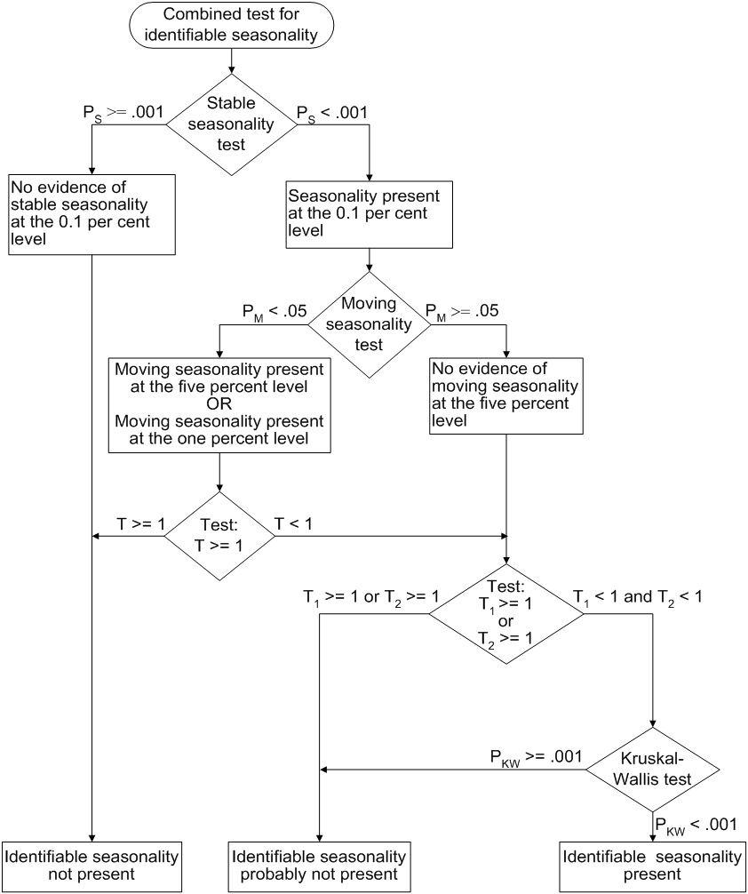
The test for identifiable seasonality is performed by combining the F tests for stable and moving seasonality, along with a Kruskal-Wallis test for stable seasonality. The following description is based on Lothian and Morry (1978b); other details can be found in Dagum (1988, 1983).
Let  and
and  denote the F value for the stable and moving seasonality tests, respectively. The combined test is performed as shown in Figure 43.5 and as follows:
-
If the null hypothesis of no stable seasonality is not rejected at the 0.10% significance level (
 ), then the series is considered to be nonseasonal. PROC X11 returns the conclusion, "Identifiable Seasonality Not Present."
-
If the null hypothesis in step 1 is rejected, then PROC X11 computes the following quantities:
![\[ T_{1} = \frac{7}{F_{s}} \]](images/etsug_x110075.png)
![\[ T_{2} = \frac{3F_{m}}{F_{s}} \]](images/etsug_x110076.png)
Let T denote the simple average of
 and
and  :
:
![\[ T = \frac{(T_{1}+T_{2})}{2} \]](images/etsug_x110079.png)
If the null hypothesis of no moving seasonality is rejected at the 5.0% significance level (
 ) and if
  , the null hypothesis of identifiable seasonality not present is not rejected and PROC X11 returns the conclusion, "Identifiable Seasonality Not Present."
-
If the null hypothesis of identifiable seasonality not present has not been accepted, but
 ,
,  , or the Kruskal-Wallis chi-squared test fails to reject at the 0.10% significance level (
 ), then PROC X11 returns the conclusion "Identifiable Seasonality Probably Not Present."
-
If the null hypotheses of no stable seasonality associated with the
 and Kruskal-Wallis chi-squared tests are rejected and if none of the combined measures described in steps 2 and 3 fail, then
the null hypothesis of identifiable seasonality not present is rejected and PROC X11 returns the conclusion "Identifiable Seasonality Present."
and Kruskal-Wallis chi-squared tests are rejected and if none of the combined measures described in steps 2 and 3 fail, then
the null hypothesis of identifiable seasonality not present is rejected and PROC X11 returns the conclusion "Identifiable Seasonality Present."
Figure 43.5: Combined Seasonality Test Flowchart
Tables Written to the OUT= Data Set
All tables that are time series can be written to the OUT= data set. However, depending on the specified options and statements, not all tables are computed. When a table is not computed, but is requested in the OUTPUT statement, the resulting variable has all missing values.
For example, if the PMFACTOR= option is not specified, Table A2 is not computed, and requesting this table in the OUTPUT statement results in the corresponding variable having all missing values.
The trading-day regression results, Tables B15 and C15, although not written to the OUT= data set, can be written to an output data set; see the OUTTDR= option for details.
Printed Output Generated by Sliding Spans Analysis
Table S 0.A
Table S 0.A gives the variable name, the length and number of spans, and the beginning and ending dates of each span.
Table S 0.B
Table S 0.B gives the summary of the two F tests performed during the standard X11 seasonal adjustments for stable and moving seasonality on Table D8, the final SI ratios. These tests are described in the section Printed Output.
Table S 1.A
Table S 1.A gives the range analysis of seasonal factors. This includes the means for each month (or quarter) within a span, the maximum percentage difference across spans for each month, and the average. The minimum and maximum within a span are also indicated.
For example, for a monthly series and an analysis with four spans, the January row would contain a column for each span, with the value representing the average seasonal factor (Table D10) over all January calendar months occurring within the span. Beside each span column is a character column with either a MIN, MAX, or blank value, indicating which calendar month had the minimum and maximum value over that span.
Denote the average over the jth calendar month in span  , by
, by  ; then the maximum percent difference (MPD) for month j is defined by
![\[ MPD_{j} = \frac{max_{k=1,..,4}\bar{S}_{j}(k) - min_{k=1,..,4}\bar{S}_{j}(k)}{min_{k=1,..,4}\bar{S}_{j}(k) } \]](images/etsug_x110088.png)
The last numeric column of Table S 1.A is the average value over all spans for each calendar month, with the minimum and maximum row flagged as in the span columns.
Table S 1.B
Table S 1.B gives a summary of range measures for each span. The first column, Range Means, is calculated by computing the maximum and minimum over all months or quarters in a span, then taking the difference. The next column is the range ratio means, which is simply the ratio of the previously described maximum and minimum. The next two columns are the minimum and maximum seasonal factors over the entire span, while the range sf column is the difference of these. Finally, the last column is the ratio of the Max SF and Min SF columns.
Breakdown Tables
Table S 2.A.1 begins the breakdown analysis for the various series considered in the sliding spans analysis. The key concept here is the MPD described above in the section Table S 1.A and in the section Computational Details for Sliding Spans Analysis. For a month or quarter that appears in two or more spans, the maximum percentage difference is computed and tested against a cutoff level. If it exceeds this cutoff, it is counted as an instance of exceeding the level. It is of interest to see if such instances fall disproportionately in certain months and years. Tables S 2.A.1 through S 6.A.3 display this breakdown for all series considered.
Table S 2.A.1
Table S 2.A.1 gives the monthly (quarterly) breakdown for the seasonal factors (table D10). The first column identifies the month or quarter. The next column is the number of times the MPD for D10 exceeded 3.0%, followed by the total count. The last is the average maximum percentage difference for the corresponding month or quarter.
Table S 2.A.2
Table S 2.A.2 gives the same information as Table S 2.A.1, but on a yearly basis.
Table S 2.A.3
The description of Table S 2.A.3 requires the definition of "Sign Change" and "Turning Point."
First, some motivation. Recall that for a highly stable series, adding or deleting a small number of observations should not affect the estimation of the various components of a seasonal adjustment procedure.
Consider Table D10, the seasonal factors in a sliding spans analysis that uses four spans. For a given observation t, looking across the four spans, we can easily pick out large differences if they occur. More subtle differences can occur when estimates go from above to below (or vice versa) a base level. In the case of multiplicative model, the seasonal factors have a base level of 100.0. So it is useful to enumerate those instances where both a large change occurs (an MPD value exceeding 3.0%) and a change of sign (with respect to the base) occur.
Let B denote the base value (which in general depends on the component being considered and the model type, multiplicative or additive).
If, for span 1,  (1) is below B (i.e.,
  is negative) and for some subsequent span k,
  is above B (i.e.,
  is positive), then a positive "Change in Sign" has occurred at observation t. Similarly, if, for span 1, (1) is above B, and for some subsequent span k, is below B, then a negative "Change in Sign" has occurred. Both cases, positive or negative, constitute a "Change in Sign"; the actual
direction is indicated in tables S 7.A through S 7.E, which are described below.
is positive), then a positive "Change in Sign" has occurred at observation t. Similarly, if, for span 1, (1) is above B, and for some subsequent span k, is below B, then a negative "Change in Sign" has occurred. Both cases, positive or negative, constitute a "Change in Sign"; the actual
direction is indicated in tables S 7.A through S 7.E, which are described below.
Another behavior of interest occurs when component estimates increase then decrease (or vice versa) across spans for a given observation. Using the preceding example, the seasonal factors at observation t could first increase, then decrease across the four spans.
This behavior, combined with an MPD exceeding the level, is of interest in questions of stability.
Again, consider Table D10, the seasonal factors in a sliding spans analysis that uses four spans. For a given observation t (containing at least three spans), note the level of D10 for the first span. Continue across the spans until a difference of 1.0% or greater occurs (or no more spans are left), noting whether the difference is up or down. If the difference is up, continue until a difference of 1.0% or greater occurs downward (or no more spans are left). If such an up-down combination occurs, the observation is counted as an up-down turning point. A similar description occurs for a down-up turning point. Tables S 7.A through S 7.E, described below, show the occurrence of turning points, indicating whether up-down or down-up. Note that it requires at least three spans to test for a turning point. Hence Tables S 2.A.3 through S 6.A.3 show a reduced number in the "Turning Point" row for the "Total Tested" column, and in Tables S 7.A through S 7.E, the turning points symbols can occur only where three or more spans overlap.
With these descriptions of sign change and turning point, we now describe Table S 2.A.3. The first column gives the type or category, the second column gives the total number of observations falling into the category, the third column gives the total number tested, and the last column gives the percentage for the number found in the category.
The first category (row) of the table is for flagged observations—that is, those observations where the MPD exceeded the appropriate cutoff level (3.0% is default for the seasonal factors). The second category is for level changes, while the third category is for turning points. The fourth category is for flagged sign changes—that is, for those observations that are sign changes, how many are also flagged. Note the total tested column for this category equals the number found for sign change, reflecting the definition of the fourth category.
The fifth column is for flagged turning points—that is, for those observations that are turning points, how many are also flagged.
The footnote to Table S 2.A.3 gives the U.S. Census Bureau recommendation for thresholds, as described in the section Computational Details for Sliding Spans Analysis.
Table S 2.B
Table S 2.B gives the histogram of flagged for seasonal factors (Table D10) using the appropriate cutoff value (default 3.0%). This table looks at the spread of the number of times the MPD exceeded the corresponding level. The range is divided up into four intervals: 3.0%–4.0%, 4.0%–5.0%, 5.0%–6.0%, and greater than 6.0%. The first column shows the symbol used in Table S 7.A, the second column gives the range in interval notation, and the last column gives the number found in the corresponding interval. Note that the sum of the last column should agree with the "Number Found" column of the "Flagged MPD" row in Table S 2.A.3.
Table S 2.C
Table S 2.C gives selected percentiles for the MPD for the seasonal factors (Table D10).
Tables S 3.A.1 through S 3.A.3
These table relate to the trading-day factors (Table C18) and follow the same format as Tables S 2.A.1 through S 2.A.3. The only difference between these tables and Tables S 2.A.1 through S 2.A.3 is the default cutoff value of 2.0% instead of the 3.0% used for the seasonal factors.
Tables S 3.B, S 3.C
These tables, applied to the trading-day factors (Table C18), are the same format as Tables S 2.B through S 2.C. The default cutoff value is different, with corresponding differences in the intervals in S 3.B.
Tables S 4.A.1 through S 4.A.3
These tables relate to the seasonally adjusted series (Table D11) and follow the same format as Tables S 2.A.1 through S 2.A.3. The same default cutoff value of 3.0% is used.
Tables S 4.B, S 4.C
These tables, applied to the seasonally adjusted series (Table D11), are the same format as tables S 2.B through S 2.C.
Tables S 5.A.1 through S 5.A.3
These table relate to the month-to-month (or quarter-to-quarter) differences in the seasonally adjusted series, and follow the same format as Tables S 2.A.1 through S 2.A.3. The same default cutoff value of 3.0% is used.
Tables S 5.B, S 5.C
These tables, applied to the month-to-month (or quarter-to-quarter) differences in the seasonally adjusted series, are the same format as tables S 2.B through S 2.C. The same default cutoff value of 3.0% is used.
Tables S 6.A.1 through S 6.A.3
These table relate to the year-to-year differences in the seasonally adjusted series, and follow the same format as Tables S 2.A.1 through S 2.A.3. The same default cutoff value of 3.0% is used.
Tables S 6.B, S 6.C
These tables, applied to the year-to-year differences in the seasonally adjusted series, are the same format as tables S 2.B through S 2.C. The same default cutoff value of 3.0% is used.
Table S 7.A
Table S 7.A gives the entire listing of the seasonal factors (Table D10) for each span. The first column gives the date for each observation included in the spans. Note that the dates do not cover the entire original data set. Only those observations included in one or more spans are listed.
The next N columns (where N is the number of spans) are the individual spans starting at the earliest span. The span columns are labeled by their beginning and ending dates.
Following the last span is the "Sign Change" column. As explained in the description of Table S 2.A.3, a sign change occurs at a given observation when the seasonal factor estimates go from above to below, or below to above, a base level. For the seasonal factors, 100.0 is the base level for the multiplicative model, 0.0 for the additive model. A blank value indicates no sign change, a "U" indicates a movement "upward" from the base level and a "D" indicates a movement "downward" from the base level.
The next column is the "Turning Point" column. As explained in the description of Table S 2.A.3, a turning point occurs when there is an upward then downward movement, or downward then upward movement, of sufficient magnitude. A blank value indicates no turning point, a "U-D" indicates a movement "upward then downward," and a "D-U" indicates a movement "downward then upward."
The next column is the maximum percentage difference (MPD). This quantity, described in the section Computational Details for Sliding Spans Analysis, is the main computation for sliding spans analysis. A measure of how extreme the MPD value is given in the last column, the "Level of Excess" column. The symbols used and their meaning are described in Table S 2.A.3. If a given observation has exceeded the cutoff, the level of excess column is blank.
Table S 7.B
Table S 7.B gives the entire listing of the trading-day factors (Table C18) for each span. The format of this table is exactly like that of Table S 7.A.
Table S 7.C
Table S 7.C gives the entire listing of the seasonally adjusted data (Table D11) for each span. The format of this table is exactly like that of Table S 7.A except for the "Sign Change" column, which is not printed. The seasonally adjusted data have the same units as the original data; there is no natural base level as in the case of a percentage. Hence the sign change is not appropriate for D11.
Table S 7.D
Table S 7.D gives the entire listing of the month-to-month (or quarter-to-quarter) changes in seasonally adjusted data for each span. The format of this table is exactly like that of Table S 7.A.
Table S 7.E
Table S 7.E gives the entire listing of the year-to-year changes in seasonally adjusted data for each span. The format of this table is exactly like that of Table S 7.A.
Printed Output from the ARIMA Statement
The information printed by default for the ARIMA model includes the parameter estimates, their approximate standard errors, t ratios, and variances, the standard deviation of the error term, and the AIC and SBC statistics for the model. In addition, a criteria summary for the chosen model is given that shows the values for each of the three test criteria and the corresponding critical values.
If the PRINTALL option is specified, a summary of the nonlinear estimation optimization and a table of Box-Ljung statistics is also produced. If the automatic model selection is used, this information is printed for each of the five predefined models. Finally, a model selection summary is printed, showing the final model chosen.