The STATESPACE Procedure

Forecasting
Given estimates of  ,
,  , and
, and  , forecasts of
  are computed from the conditional expectation of
  .
.
In forecasting, the parameters F, G, and are replaced with the estimates or by values specified in the RESTRICT statement. One-step-ahead forecasting is performed
for the observation , where  . Here
  is the number of observations and b is the value of the BACK= option. For the observation , where
  , m-step-ahead forecasting is performed for
  . The forecasts are generated recursively with the initial condition
  .
.
The m-step-ahead forecast of  is
is  , where denotes the conditional expectation of given the information available at time t. The m-step-ahead forecast of
  is
is 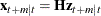 , where the matrix
 ![${\mb{H} = [\mb{I}_{r} \mb{0} ]}$](images/etsug_statespa0154.png) .
.
Let  . Note that the last
  elements of consist of the elements of
  for
for  .
.
The state vector can be represented as
![\[ \mb{z}_{t+m} = \mb{F} ^{m} \mb{z}_{t} + \sum _{i=0}^{m-1}{\bPsi _{i} \mb{e}_{t+m-i}} \]](images/etsug_statespa0158.png)
Since  for
for  , the m-step-ahead forecast is
![\[ \mb{z}_{t+m|t} = \mb{F} ^{m} \mb{z}_{t} = \mb{F} \mb{z}_{t+m-1|t} \]](images/etsug_statespa0161.png)
Therefore, the m-step-ahead forecast of is
![\[ \mb{x}_{t+m|t} = \mb{H} \mb{z}_{t+m|t} \]](images/etsug_statespa0162.png)
The m-step-ahead forecast error is
![\[ \mb{z}_{t+m}-\mb{z}_{t+m|t} = \sum _{i=0}^{m-1}{\bPsi _{i} \mb{e}_{t+m-i}} \]](images/etsug_statespa0163.png)
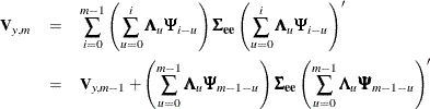
The variance of the m-step-ahead forecast error is
![\[ \mb{V}_{z,m} = \sum _{i=0}^{m-1}{\bPsi _{i} \bSigma _{\mb{ee}} {\Psi }_{i}’} \]](images/etsug_statespa0164.png)
Letting  , the variance of the m-step-ahead forecast error of ,
  , can be computed recursively as follows:
![\[ \mb{V}_{z,m} = \mb{V}_{z,m-1} + \bPsi _{m-1} \bSigma _{\mb{ee}} \bPsi ^{'}_{m-1} \]](images/etsug_statespa0167.png)
The variance of the m-step-ahead forecast error of is the  left upper submatrix of ; that is,
![\[ \mb{V}_{x,m} = \mb{H} \mb{V}_{z,m}\mb{H} ’ \]](images/etsug_statespa0168.png)
Unless the NOCENTER option is specified, the sample mean vector is added to the forecast. When differencing is specified,
the forecasts x  plus the sample mean vector are integrated back to produce forecasts for the original series.
Let  be the original series specified by the VAR statement, with some 0 values appended that correspond to the unobserved past
observations. Let B be the backshift operator, and let
be the original series specified by the VAR statement, with some 0 values appended that correspond to the unobserved past
observations. Let B be the backshift operator, and let  be the
  matrix polynomial in the backshift operator that corresponds to the differencing specified by the VAR statement. The off-diagonal
elements of
matrix polynomial in the backshift operator that corresponds to the differencing specified by the VAR statement. The off-diagonal
elements of  are 0. Note that
  , where
  is the identity matrix. Then
  .
.
This gives the relationship
![\[ \mb{y}_{t} = \bDelta ^{-1}(B) \mb{z}_{t} = \sum _{i=0}^{{\infty }}{\bLambda _{i}\mb{z}_{t-i}} \]](images/etsug_statespa0176.png)
where 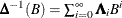 and
and  .
.
The m-step-ahead forecast of  is
is
![\[ \mb{y}_{t+m|t} = \sum _{i=0}^{m-1}{\bLambda _{i} \mb{z}_{t+m-i|t}} + \sum _{i=m}^{{\infty }}{\bLambda _{i} \mb{z}_{t+m-i}} \]](images/etsug_statespa0180.png)
The m-step-ahead forecast error of is
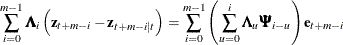
Letting  , the variance of the m-step-ahead forecast error of ,
  , is
, is