The SSM Procedure
-
Overview

- Getting Started
-
Syntax
-
DetailsState Space Model and NotationTypes of Sequence DataOverview of Model Specification SyntaxFiltering, Smoothing, Likelihood, and Structural Break DetectionEstimation of User-Specified Linear Combination of State ElementsContrasting PROC SSM with Other SAS Procedures Predefined Trend ModelsPredefined Structural ModelsModels with Dependent LagsCovariance ParameterizationMissing ValuesComputational IssuesDisplayed OutputODS Table NamesODS Graph NamesOUT= Data Set
-
ExamplesBivariate Basic Structural Model Panel Data: Random-Effects and Autoregressive ModelsBackcasting, Forecasting, and InterpolationLongitudinal Data: Smoothing of Repeated MeasuresA User-Defined Trend ModelModel with Multiple ARIMA ComponentsDynamic Factor ModelingDiagnostic Plots and Structural Break AnalysisLongitudinal Data: Variable Bandwidth SmoothingA Transfer Function Model for the Gas Furnace DataPanel Data: Dynamic Panel Model for the Cigar DataMultivariate Modeling: Long-Term Temperature TrendsBivariate Model: Sales of Mink and Muskrat FursFactor Model: Now-Casting the US EconomyLongitudinal Data: Lung Function Analysis
- References
Multivariate Season
The STATE statement option TYPE=SEASON(LENGTH=s)
specifies a ((s–1)*dim)-dimensional  , needed for defining a dim-dimensional trigonometric season component with season length s. A (multivariate) trigonometric season component,
  , is a sum of (multivariate) cycles of different frequencies,
![\[ \pmb {\zeta } = \sum _{j = 1}^{[s/2]} \pmb {\zeta }_{j} \]](images/etsug_ssm0417.png)
where the constituent cycles  , called harmonics, have frequencies
  s. All the harmonics are assumed to be statistically independent, have the same damping factor
  , and are governed by the disturbances with the same covariance matrix
  . The number of harmonics,
 ![$[\Argument{s}/2]$](images/etsug_ssm0419.png) , equals
, equals  if s is even and
  if it is odd. This means that specifying TYPE=SEASON(LENGTH=s)
is equivalent to specifying cycle specifications with correct frequencies, damping factor , and the COV
option restricted to the same covariance . The resulting is necessarily ((s–1)*dim)-dimensional. When the season length
if it is odd. This means that specifying TYPE=SEASON(LENGTH=s)
is equivalent to specifying cycle specifications with correct frequencies, damping factor , and the COV
option restricted to the same covariance . The resulting is necessarily ((s–1)*dim)-dimensional. When the season length  is even, the last harmonic cycle,
  , has frequency
  and requires special attention. It is of dimension dim rather than 2*dim because its underlying state equation simplifies to a dim-variate autoregression with autoregression coefficient
  . As a result of this discussion, it is clear that the system matrices
  and
and  associated with the ((s–1)*dim)-dimensional are block-diagonal with the blocks corresponding to the harmonics. The initial condition is fully diffuse.
For all the models discussed so far, the first dim elements of provided the needed (multivariate) component. This is not the case for the (multivariate) season component. Extracting the
ith seasonal component from requires accumulating the contributions from the harmonics that are associated with this ith seasonal, which are not organized contiguously in . For example, suppose that dim is 2 and the season length s is 4. In this case ![$[\Argument{s}/2] $](images/etsug_ssm0427.png) is 2, and the bivariate seasonal component is a sum of two independent bivariate cycles,
is 2, and the bivariate seasonal component is a sum of two independent bivariate cycles,  and
and  . The cycle
  has frequency
  and its underlying state, say
  , has dimension
  . The last harmonic,
  , has frequency , and therefore its underlying state, say
  , has dimension 2. The combined state
  has dimension
  . In order to extract the first bivariate seasonal component, you must extract the first components of bivariate cycles and , which in turn implies the first elements of
  and
and  , respectively. Thus, obtaining the first bivariate seasonal component requires extracting the first and the fifth elements
of the combined state
, respectively. Thus, obtaining the first bivariate seasonal component requires extracting the first and the fifth elements
of the combined state  . Similarly, obtaining the second bivariate seasonal component requires extracting the second and the sixth elements of the
combined state . All this can be summarized by the dot product expressions
. Similarly, obtaining the second bivariate seasonal component requires extracting the second and the sixth elements of the
combined state . All this can be summarized by the dot product expressions
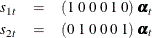
where  and
and  denote the first and second components, respectively, of the bivariate seasonal component. Note that and are univariate seasonal components, each of season length 4, in their own right. They are correlated components; their correlation
structure depends on .
denote the first and second components, respectively, of the bivariate seasonal component. Note that and are univariate seasonal components, each of season length 4, in their own right. They are correlated components; their correlation
structure depends on .
Obtaining the desired components of the multivariate seasonal component is made easy by a special syntax convention of the
COMPONENT statement. Continuing with the previous example, the following examples illustrate two equivalent ways of obtaining
and . The first set of statements explicitly specify the linear combinations needed for defining and :
     state seasonState(2) type=season(length=4)  ...;
     component s_1 =( 1  0  0  0  1  0 ) * seasonState;
     component s_2 =( 0  1  0  0  0  1 ) * seasonState;
The following simpler specification achieves the same result:
     state seasonState(2) type=season(length=4)  ...;
     component s_1 = seasonState[1];
     component s_2 = seasonState[2];
In the latter specification, the meaning of the element operator [] changes if the state in question is defined by using the TYPE= option.