The SSM Procedure
-
Overview

- Getting Started
-
Syntax
-
DetailsState Space Model and NotationTypes of Sequence DataOverview of Model Specification SyntaxFiltering, Smoothing, Likelihood, and Structural Break DetectionEstimation of User-Specified Linear Combination of State ElementsContrasting PROC SSM with Other SAS Procedures Predefined Trend ModelsPredefined Structural ModelsModels with Dependent LagsCovariance ParameterizationMissing ValuesComputational IssuesDisplayed OutputODS Table NamesODS Graph NamesOUT= Data Set
-
ExamplesBivariate Basic Structural Model Panel Data: Random-Effects and Autoregressive ModelsBackcasting, Forecasting, and InterpolationLongitudinal Data: Smoothing of Repeated MeasuresA User-Defined Trend ModelModel with Multiple ARIMA ComponentsDynamic Factor ModelingDiagnostic Plots and Structural Break AnalysisLongitudinal Data: Variable Bandwidth SmoothingA Transfer Function Model for the Gas Furnace DataPanel Data: Dynamic Panel Model for the Cigar DataMultivariate Modeling: Long-Term Temperature TrendsBivariate Model: Sales of Mink and Muskrat FursFactor Model: Now-Casting the US EconomyLongitudinal Data: Lung Function Analysis
- References
Multivariate Cycle
The STATE statement option TYPE=CYCLE
specifies a (2*dim)-dimensional  , needed for defining a dim-dimensional cycle. As in the LL case, the first dim elements of correspond to the needed dim-dimensional cycle, and the remaining dim elements contain some auxiliary quantities. The cycle model defined in this subsection requires a regular data type—that
is, the CT option is not included. Let
, needed for defining a dim-dimensional cycle. As in the LL case, the first dim elements of correspond to the needed dim-dimensional cycle, and the remaining dim elements contain some auxiliary quantities. The cycle model defined in this subsection requires a regular data type—that
is, the CT option is not included. Let  denote the damping factor, and let
  period be the frequency associated with the cycle. The admissible parameter ranges are
  and period
  , which implies that
  . Let
. Let  , a
, a  matrix, and let
  , a
, a  matrix. With this notation, the transition equation associated with is
![\[ \pmb {\alpha }_{t+1} = \mb{T} \pmb {\alpha }_{t} + \pmb {\eta }_{t+1} \]](images/etsug_ssm0398.png)
where  is a sequence of zero mean, independent,
  -dimensional Gaussian vectors with covariance
  . If
. If  , the initial condition is fully diffuse (
 and
and  ). Otherwise, it is nondiffuse:
 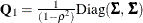 and
and  .
.
The multivariate cycle is useful for capturing periodic behavior for multivariate time series data. The cycle term for the
ith response variable is defined by a component that simply picks the ith element of . For example, the component cycle_i defined as follows can be used as a cycle term in the MODEL statement of the ith response variable:
     state cycleState(dim) type=cycle  ...;
     component cycle_2 = cycleState[2];