The HPQLIM Procedure

Ordinal Discrete Choice Modeling
Binary Probit and Logit Model
The binary choice model is
![\[ y^{*}_{i} = \mathbf{x}_{i}’\bbeta + \epsilon _{i} \]](images/etsug_hpqlim0003.png)
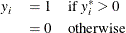
where the value of the latent dependent variable,  , is observed only as follows:
The disturbance,  , of the probit model has a standard normal distribution with the distribution function (CDF)
![\[ \Phi (x)=\int _{-\infty }^{x}\frac{1}{\sqrt {2\pi }}\exp (-t^2/2)dt \]](images/etsug_hpqlim0062.png)
The disturbance of the logit model has a standard logistic distribution with the distribution function (CDF)
![\[ \Lambda (x)=\frac{\exp (x)}{1+\exp (x)} = \frac{1}{1+\exp (-x)} \]](images/etsug_hpqlim0063.png)
The binary discrete choice model has the following probability that the event  occurs:
![\[ P(y_{i}=1) = F(\mathbf{x}_{i}’\bbeta ) = \left\{ \begin{array}{ll} \Phi (\mathbf{x}_{i}’\bbeta ) & \mr{(probit)} \\ \Lambda (\mathbf{x}_{i}’\bbeta ) & \mr{(logit)} \end{array} \right. \]](images/etsug_hpqlim0065.png)
For more information, see the section Ordinal Discrete Choice Modeling.
Ordinal Probit/Logit
When the dependent variable is observed in sequence with M categories, binary discrete choice modeling is not appropriate for data analysis. McKelvey and Zavoina (1975) propose the ordinal (or ordered) probit model.
Consider the regression equation
![\[ y_{i}^{*} = \mathbf{x}_{i}’\bbeta + \epsilon _{i} \]](images/etsug_hpqlim0066.png)
where error disturbances, , have the distribution function F. The unobserved continuous random variable,  , is identified as M categories. Suppose there are
  real numbers,
  , where
  ,
,  ,
,  , and
, and 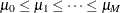 . Define
![\[ R_{i,j} = \mu _{j} - \mathbf{x}_{i}’\bbeta \]](images/etsug_hpqlim0074.png)
The probability that the unobserved dependent variable is contained in the jth category can be written as
![\[ P[\mu _{j-1}< y_{i}^{*} \leq \mu _{j}] = F(R_{i,j}) - F(R_{i,j-1}) \]](images/etsug_hpqlim0075.png)
For more information, see the section Ordinal Discrete Choice Modeling.